

Naive Bayes Classification
This section introduces Naive Bayes, the classifier behind many spam filters. It turns counts from the training data into probabilities with Bayes' theorem, then picks the class with the highest probability. You will first run the method by hand on real counts from 999 e-mails, then build a spam filter and a wine classifier in scikit-learn with the two notebooks of week 7.
Objectives
By the end of the section you should be able to:
- State Bayes' theorem and name its four parts: prior, likelihood, evidence and posterior.
- Compute the probability that an e-mail is spam given one word, from real counts.
- Explain the naive assumption and use it to score an e-mail word by word, by hand.
- Explain why a word count of 0 breaks the model and how Laplace smoothing (
alpha=1) fixes it. - Build, evaluate and use a
MultinomialNBspam filter withCountVectorizer. - Explain how
GaussianNBhandles numeric features, and train it on the wine data.
Where this sits in the course
Week 7 of the plan has three parts:
- Two notebooks.
E-Mail Classificationbuilds a spam filter from 1000 labelled e-mails.Naive_Bayes_Classificationclassifies wines from their chemical analysis. - A real-world scenario. Spam e-mail detection: decide from its words whether an e-mail is spam or a legitimate e-mail (called ham).
- A project milestone. Machine Learning Model Implementation: this week your team adds a Naive Bayes model on its own data.
In weeks 4 to 6 you trained logistic regression, KNN, decision trees and random forests with the same fit, predict and score pattern, and read confusion matrices. Naive Bayes uses the same pattern. What is new is the idea inside the model: it counts, and it multiplies probabilities.
| Part | What we do | Time |
|---|---|---|
| 1 | Bayes' theorem, and one word by hand | 20 min |
| 2 | Naive Bayes by hand, and smoothing | 30 min |
| 3 | Notebook 1: the spam filter | 20 min |
| 4 | Notebook 2: Gaussian Naive Bayes on wine | 20 min |
| 5 | Practice with answers, then takeaways | 30 min |
Part 1: Bayes' theorem
Conditional probability
A conditional probability is the probability that something will happen, given that something else has already occurred. We write it with a vertical bar:
P(A | B) = the probability of A, given that B is trueFor e-mails: P(S | m) is the probability that an e-mail is spam (S) given that it contains the word money (m). The reverse, P(m | S), is the probability that an e-mail contains money given that it is spam. These are two different numbers.
Bayes' theorem
Bayes' theorem connects the two directions:
P(A | B) = P(B | A) P(A) / P(B)For a class c and some evidence x about the e-mail:
| Part | Symbol | Meaning |
|---|---|---|
| Prior | P(c) | how common the class is before we look at the e-mail |
| Likelihood | P(x | c) | how common the evidence is inside that class |
| Evidence | P(x) | how common the evidence is overall |
| Posterior | P(c | x) | the probability of the class after seeing the evidence |
The likelihood is easy to count from labelled data: look only at the spam e-mails and count. The posterior is what we want. Bayes' theorem turns the first into the second.
Worked example: spam, given the word money
The notebook's dataset holds 999 e-mails once a duplicate is removed: 500 spam and 499 ham. We count how many of them contain the word money at least once.
| Class | E-mails | Containing money |
|---|---|---|
Spam S | 500 | 79 |
Ham H | 499 | 25 |
| All | 999 | 104 |
Question: a new e-mail contains money. What is P(S | m)?
Step 1: the prior and the likelihood
Both come straight from the table:
P(S)     = 500 / 999 = 0.5005
P(m | S) = 79 / 500  = 0.158
Step 2: the evidence
P(m) counts the word in all e-mails, spam and ham together:
P(m) = (79 + 25) / 999 = 104 / 999 = 0.1041Step 3: the posterior
P(S | m) = P(m | S) P(S) / P(m) = 0.158 x 0.5005 / 0.1041 = 0.7596Seeing money raises the probability of spam from about one half to about three quarters. Check: among the 104 e-mails that contain money, 79 are spam, and 79 / 104 = 0.7596, the same answer. Bayes' theorem gives exactly what direct counting gives. Its value is that it still works when we cannot count directly, which is the case as soon as we look at many words at once.
Part 2: Naive Bayes by hand
From one word to many: the naive assumption
An e-mail has many words x1, x2, ..., xn. Bayes' theorem for the whole e-mail needs P(x1, x2, ..., xn | c), the probability of this exact combination of words inside a class. Almost no combination appears twice in 999 e-mails, so it cannot be counted.
Naive Bayes assumes that the words are conditionally independent given the class: once we know an e-mail is spam, seeing one word tells us nothing more about the next word. Then the joint likelihood is a product of one-word likelihoods:
P(x1, x2, ..., xn | c) = P(x1 | c) x P(x2 | c) x ... x P(xn | c)This is why it is called naive. Real words are not independent (order and online often come together in spam), but the method performs surprisingly well even when the assumption does not hold. Training is also fast: no weights are fitted by an optimization procedure, the model only counts.
The classification rule
P(x1, ..., xn) is the same for every class, so it does not change which class wins. The rule is:
- For every class
c, compute the scoreP(c) x P(x1 | c) x ... x P(xn | c). - Predict the class with the largest score.
- To report probabilities, normalize: divide each score by the sum of all scores. That is what
predict_probaprints.
The prior P(c) is the fraction of training e-mails in class c.
Counting words: MultinomialNB
The spam notebook uses MultinomialNB, which works on word counts. The probability of word w in class c is the share of the class's words that are w:
P(w | c) = (n_wc + alpha) / (N_c + alpha x V)n_wc: how many timeswappears in all training e-mails of classcN_c: the total count of all vocabulary words in classcV: the number of words in the vocabularyalpha: the smoothing value.MultinomialNB()usesalpha=1.0by default; we explain it at the end of this part.
A word that appears twice in an e-mail enters the product twice.
Worked example: a four-word spam filter
To keep the numbers small, imagine a filter whose vocabulary is only four words: money, online, meeting and meds. These are their real counts in the 999 e-mails:
| Word | Count in ham | Count in spam |
|---|---|---|
money | 38 | 155 |
online | 7 | 94 |
meeting | 153 | 1 |
meds | 0 | 30 |
Total N_c | 198 | 280 |
The priors are P(H) = 499 / 999 = 0.4995 and P(S) = 500 / 999 = 0.5005, and V = 4, alpha = 1.
The e-mail to classify is the spam test message from the notebook:
Why pay more for expensive meds when you can order them online and save $$$?Step 1: which words does the filter see?
Only vocabulary words count. The message contains meds once and online once; every other word (why, pay, order, save...) is ignored because it is not in the vocabulary. CountVectorizer does exactly the same with its own, much bigger, vocabulary.
Step 2: the word probabilities
With alpha = 1, each denominator is N_c + 4: 202 for ham and 284 for spam.
| Word | P(w | H) | P(w | S) |
|---|---|---|
online | (7 + 1) / 202 = 0.0396 | (94 + 1) / 284 = 0.3345 |
meds | (0 + 1) / 202 = 0.00495 | (30 + 1) / 284 = 0.1092 |
Both words are far more likely in spam than in ham.
Step 3: the two scores
score(H) = 0.4995 x 0.0396 x 0.00495 = 0.0000979
score(S) = 0.5005 x 0.3345 x 0.1092  = 0.0183
The spam score is about 187 times the ham score.
Step 4: normalize
P(S | e-mail) = 0.0183 / (0.0183 + 0.0000979) = 0.9947
P(H | e-mail) = 1 - 0.9947 = 0.0053
The prediction is spam. As a check, MultinomialNB() trained on the same four-word count matrix (CountVectorizer(vocabulary=['money', 'online', 'meeting', 'meds'])) prints [0.00533, 0.99467] from predict_proba for this message.
Open the spam filter widget full screen to watch this example build up word by word. Switch to All 8052 words to run the same message through a filter trained on every word that appears in at least two of the 999 e-mails, with English stop words removed.
The zero-count problem and Laplace smoothing
A new e-mail arrives:
Money for the meeting? The meeting is about meds.It contains money once, meeting twice and meds once. meeting is a strong ham word (153 times in ham, once in spam), so we expect ham.
Without smoothing (alpha = 0), P(w | c) = n_wc / N_c. The word meds never appears in the 499 ham e-mails, so:
P(meds | H) = 0 / 198 = 0
score(H) = 0.4995 x 0.1919 x 0.7727 x 0.7727 x 0 = 0
One zero wipes out the whole product. The ham score is exactly 0, so P(S | e-mail) = 1: the model is completely sure the e-mail is spam, and the two meeting words count for nothing.
With Laplace smoothing (alpha = 1), every count gets one extra, so no word probability is ever 0:
| Word | P(w | H) | P(w | S) |
|---|---|---|
money | 39 / 202 = 0.1931 | 156 / 284 = 0.5493 |
meeting | 154 / 202 = 0.7624 | 2 / 284 = 0.00704 |
meds | 1 / 202 = 0.00495 | 31 / 284 = 0.1092 |
score(H) = 0.4995 x 0.1931 x 0.7624 x 0.7624 x 0.00495 = 0.0002775
score(S) = 0.5005 x 0.5493 x 0.00704 x 0.00704 x 0.1092 = 0.000001488
P(H | e-mail) = 0.0002775 / (0.0002775 + 0.000001488) = 0.9947
Now the prediction is ham, with probability 0.9947, which matches predict_proba on the four-word model. MultinomialNB() smooths with alpha=1.0 unless you set another value. With a real vocabulary of thousands of words, a word that never appeared in one class is the normal case, not the exception, so smoothing is essential. In the widget, switch smoothing to 0 and pick The zero-count e-mail to see the posterior jump to 1 on the word meds.
Part 3: Notebook 1, the spam filter
Open the notebook
Open E-Mail Classification in Colab
The first code cell reads Data/ham-spam.csv, a folder that does not exist next to the notebook in Colab. Read the file from the repository instead:
import pandas as pd

url = ("https://raw.githubusercontent.com/"
       "jeffprosise/Machine-Learning/master/Data/ham-spam.csv")
df = pd.read_csv(url)
df.head()
Load the data and remove the duplicate
df.info() reports 1000 rows and two columns: IsSpam (0 for ham, 1 for spam) and Text, already lower-cased and stripped of punctuation. No values are missing.
df.groupby('IsSpam').describe()
df = df.drop_duplicates()
df.groupby('IsSpam').describe()
The first describe() shows 500 ham e-mails but only 499 unique ones: one ham e-mail appears twice. After drop_duplicates() the data has 999 rows: 499 ham and 500 spam, still balanced.
Turn text into counts: CountVectorizer
A model cannot use text directly, so each e-mail becomes a row of word counts:
from sklearn.feature_extraction.text import CountVectorizer

vectorizer = CountVectorizer(ngram_range=(1, 2), stop_words='english')
x = vectorizer.fit_transform(df['Text'])
y = df['IsSpam']fit_transformbuilds the vocabulary from all e-mails and returns a sparse matrix of counts: one row per e-mail, one column per vocabulary entry.ngram_range=(1, 2)keeps single words and pairs of neighbouring words, such asorder online.stop_words='english'drops very common words such asthe,forandyou.x.shapeis(999, 100687): the vocabulary has 100687 entries.
Worked example: what the vectorizer keeps
The notebook transforms a messy sentence and turns it back into words to show the cleaning:
text = vectorizer.transform(['Why pay MORE for * expensive meds when you can ...123... order them online and save $$$?'])
text = vectorizer.inverse_transform(text)
print(text)
Before running it, predict which words survive. The output:
[array(['expensive', 'meds', 'online', 'order', 'order online', 'pay',
       'save'], dtype='<U401')]
MORE was lower-cased and then dropped as a stop word, as were why, for, when, you, can, them and and. The symbols and 123 are gone. The pair order online was kept because it appeared in the training e-mails.
Split and train
from sklearn.model_selection import train_test_split
x_train, x_test, y_train, y_test = train_test_split(x, y, test_size=0.2, random_state=0)

from sklearn.naive_bayes import MultinomialNB
model = MultinomialNB()
model.fit(x_train, y_train)
test_size=0.2 keeps 200 e-mails for testing (102 ham, 98 spam) and trains on 799. fit does nothing more than the counting of Part 2: the priors and, for every one of the 100687 columns, the smoothed probability in each class.
The confusion matrix
The notebook imports plot_confusion_matrix, which was removed from scikit-learn in version 1.2, so that cell fails today with an ImportError. Use the replacement:
from sklearn.metrics import ConfusionMatrixDisplay

ConfusionMatrixDisplay.from_estimator(model, x_test, y_test,
    display_labels=['Not Spam', 'Spam'], cmap='Blues', xticks_rotation='vertical')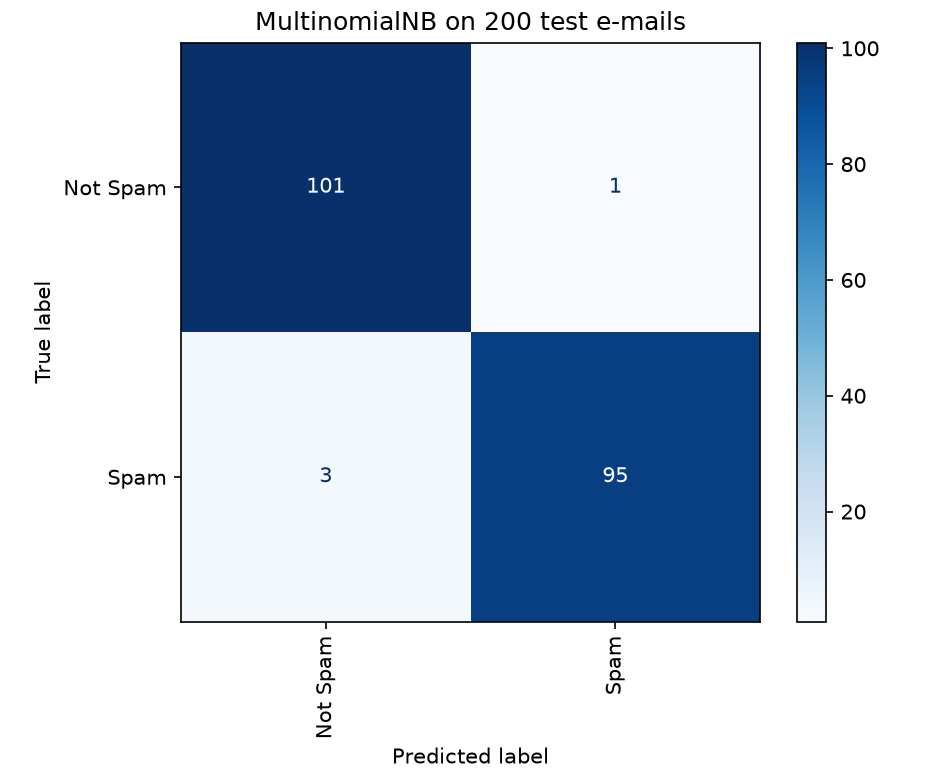
Rows are the true class and columns the prediction. The model identified 101 of 102 ham e-mails as not spam, and 95 of 98 spam e-mails as spam.
Worked example: score the spam filter
From the matrix:
accuracy          = (101 + 95) / 200 = 0.98
precision (spam)  = 95 / (95 + 1)    = 0.9896
recall (spam)     = 95 / (95 + 3)    = 0.9694
model.score(x_test, y_test) prints 0.98. Precision tells us that when the filter says spam it is almost always right: only one legitimate e-mail went to the spam folder. Recall tells us it catches 97 percent of the spam.
The notebook then measures the area under the ROC curve from the predicted probabilities:
from sklearn.metrics import roc_auc_score

probabilities = model.predict_proba(x_test)
roc_auc_score(y_test, probabilities[:, 1])
The output is 0.9992997198879552, very close to the perfect value of 1.
Classify new e-mails
message = vectorizer.transform(['Can you attend a code review on Tuesday? Need to make sure the logic is rock solid.'])
model.predict(message)[0]
model.predict_proba(message)[0][0]
predict returns 0 (not spam), and the probability of not spam is 0.9999170457201042. For the spam message:
message = vectorizer.transform(['Why pay more for expensive meds when you can order them online and save $$$?'])
model.predict(message)[0]
model.predict_proba(message)[0][1]
predict returns 1 (spam), with a spam probability of 0.9997857610873945. predict_proba returns two values per e-mail, the probability of class 0 and of class 1, in that order.
Part 4: Notebook 2, Gaussian Naive Bayes on wine
Open the notebook
Open Naive_Bayes_Classification in Colab
The notebook reads ./Datasets/wine.data.csv, which is not next to it in Colab. Read it from the repository:
import numpy as np
import pandas as pd
import matplotlib.pyplot as plt

url = ("https://raw.githubusercontent.com/tirthajyoti/"
       "Machine-Learning-with-Python/master/Datasets/wine.data.csv")
df = pd.read_csv(url)
The wine data
The data holds 178 wines grown in the same region of Italy but from three different cultivars, the column Class with values 1, 2 and 3 (59, 71 and 48 wines). The other 13 columns are the quantities of constituents found by chemical analysis, such as Alcohol, Flavanoids and Proline. All 13 features are numbers, not word counts.
The notebook draws one boxplot per feature, split by class:
for c in df.columns[1:]:
    df.boxplot(c, by='Class', figsize=(7, 4), fontsize=14)
    plt.title("{}\n".format(c), fontsize=16)
    plt.xlabel("Wine Class", fontsize=16)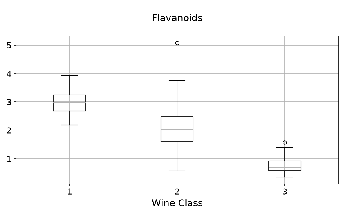
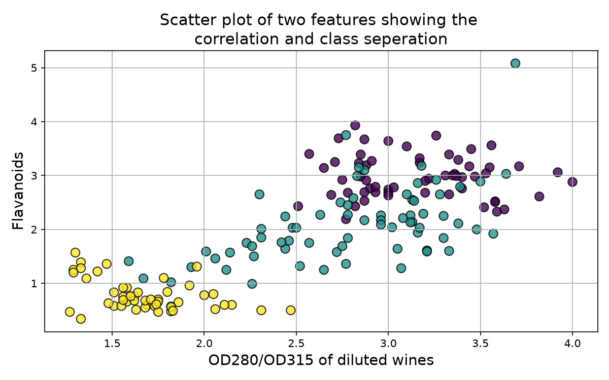
Some features separate the classes clearly. Flavanoids is high for class 1, middle for class 2 and low for class 3. The scatter plot of two features shows the picture in two dimensions: class 3 sits apart at low values of both features, while classes 1 and 2 overlap heavily.
Are the features independent?
Naive Bayes assumes the features are independent given the class. The notebook checks with a correlation matrix. Its cell calls cm.get_cmap, which recent Matplotlib versions removed, and sets the tick labels without setting the tick positions, so the labels land in the wrong places. The fixed version:
def correlation_matrix(df):
    fig = plt.figure(figsize=(16, 12))
    ax1 = fig.add_subplot(111)
    cmap = plt.get_cmap('jet', 30)
    cax = ax1.imshow(df.corr(), interpolation="nearest", cmap=cmap)
    ax1.grid(True)
    plt.title('Wine data set features correlation\n', fontsize=15)
    labels = df.columns
    ax1.set_xticks(range(len(labels)))
    ax1.set_yticks(range(len(labels)))
    ax1.set_xticklabels(labels, fontsize=9, rotation=90)
    ax1.set_yticklabels(labels, fontsize=9)
    fig.colorbar(cax, ticks=[0.1 * i for i in range(-11, 11)])
    plt.show()

correlation_matrix(df)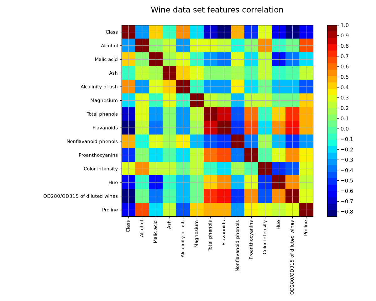
Flavanoids has a correlation of 0.86 with Total phenols and 0.79 with OD280/OD315 of diluted wines. The features are clearly not independent. The notebook applies the classifier anyway to see how it performs.
The Gaussian likelihood
Word counts suit MultinomialNB. For numeric features, GaussianNB assumes that inside each class a feature follows a bell curve (a Gaussian). For a feature value x in class c:
f(x | c) = 1 / square root(2 pi sigma_c^2) x e^( -(x - mu_c)^2 / (2 sigma_c^2) )mu_c: the mean of the feature over the training rows of classcsigma_c: the standard deviation of the feature in classc(dividing by n)f(x | c): the height of the bell curve atx, used as the likelihood
fit computes one mean and one standard deviation per feature and per class, plus the priors. The rest of the rule is the same as in Part 2: multiply the prior by the likelihoods, pick the largest, normalize.
Worked example: one wine, one feature
We use one feature, Flavanoids, over all 178 wines. Its mean and standard deviation per class:
| Class | Wines | Mean mu | Std sigma |
|---|---|---|---|
| 1 | 59 | 2.982 | 0.394 |
| 2 | 71 | 2.081 | 0.701 |
| 3 | 48 | 0.781 | 0.290 |
A new wine has Flavanoids = 2.0. Which class does Gaussian Naive Bayes predict?
Step 1: the exponent for each class
The exponent is -(x - mu)^2 / (2 sigma^2):
class 1: -(2.0 - 2.982)^2 / (2 x 0.394^2) = -0.9643 / 0.3105 = -3.106
class 2: -(2.0 - 2.081)^2 / (2 x 0.701^2) = -0.00656 / 0.9828 = -0.0067
class 3: -(2.0 - 0.781)^2 / (2 x 0.290^2) = -1.4860 / 0.1682 = -8.834
The value 2.0 is close to the class 2 mean, so its exponent is almost 0.
Step 2: the densities
Multiply e to the exponent by the factor 1 / square root(2 pi sigma^2):
f(2.0 | 1) = 1.0125 x e^(-3.106)  = 1.0125 x 0.04478  = 0.0453
f(2.0 | 2) = 0.5691 x e^(-0.0067) = 0.5691 x 0.99335  = 0.5653
f(2.0 | 3) = 1.3757 x e^(-8.834)  = 1.3757 x 0.000146 = 0.000200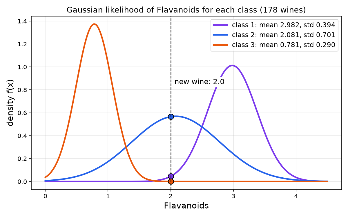
Step 3: priors, scores and the posterior
The priors are 59/178 = 0.3315, 71/178 = 0.3989 and 48/178 = 0.2697.
| Class | f(x | c) | P(c) | Score | Posterior |
|---|---|---|---|---|
| 1 | 0.0453 | 0.3315 | 0.015029 | 0.0625 |
| 2 | 0.5653 | 0.3989 | 0.22549 | 0.9373 |
| 3 | 0.000200 | 0.2697 | 0.000054 | 0.0002 |
The scores add up to 0.24057, and each posterior is its score divided by that sum. The prediction is class 2, with probability about 0.94. GaussianNB fitted on Flavanoids alone prints [0.0624, 0.9374, 0.0002]; the last digit differs because we rounded the means and standard deviations to three decimals.
Open the Gaussian Naive Bayes widget full screen. Drag across the chart to move the wine, switch the feature, and compare the priors from the data with equal priors.
Train on all 13 features
from sklearn.model_selection import train_test_split
from sklearn.naive_bayes import GaussianNB

X = df.drop('Class', axis=1)
y = df['Class']
X_train, X_test, y_train, y_test = train_test_split(X, y, test_size=0.3, random_state=0)

nbc = GaussianNB()
nbc.fit(X_train, y_train)
y_pred = nbc.predict(X_test)
mislabel = np.sum((y_test != y_pred))
print("Total number of mislabelled data points from {} test samples is {}".format(len(y_test), mislabel))
The notebook's split has no random_state, so every run draws a different split and prints a different count (its saved output shows 2). With random_state=0, as above, the split is repeatable: 124 training wines, 54 test wines, and the output is:
Total number of mislabelled data points from 54 test samples is 3The accuracy is 51 / 54 = 0.9444. The confusion matrix, confusion_matrix(y_test, y_pred):
| Predicted 1 | Predicted 2 | Predicted 3 | |
|---|---|---|---|
| Actual 1 | 19 | 0 | 0 |
| Actual 2 | 2 | 19 | 1 |
| Actual 3 | 0 | 0 | 13 |
All three mistakes are class 2 wines: two predicted as class 1 and one as class 3. The classifier does well even though its independence assumption is clearly false for these features.
A swapped report
The notebook prints classification_report(y_pred, y_test). The function expects the true labels first: classification_report(y_test, y_pred). With the arguments swapped, precision and recall trade places and support counts the predictions instead of the true classes. For class 2:
| Call | Precision | Recall | Support |
|---|---|---|---|
classification_report(y_pred, y_test) | 0.86 | 1.00 | 19 |
classification_report(y_test, y_pred) | 1.00 | 0.86 | 22 |
Check the correct row against the confusion matrix. Precision reads down the column: 19 wines were predicted as class 2, and all 19 are class 2, so 19 / 19 = 1.00. Recall reads along the row: 22 wines really are class 2, and 19 of them were found, so 19 / 22 = 0.86. The correct call prints:
              precision    recall  f1-score   support

           1       0.90      1.00      0.95        19
           2       1.00      0.86      0.93        22
           3       0.93      1.00      0.96        13

    accuracy                           0.94        54
   macro avg       0.94      0.95      0.95        54
weighted avg       0.95      0.94      0.94        54
Always pass the true labels first, to confusion_matrix and to classification_report alike.
Common mistakes
- Reading
Data/ham-spam.csvor./Datasets/wine.data.csvin Colab from a folder that does not exist there. - Calling
plot_confusion_matrix, which no longer exists. UseConfusionMatrixDisplay.from_estimator. - Setting
alpha=0: one word never seen in a class sets that class's probability to exactly 0. - Calling
fit_transformon new e-mails. New text needsvectorizer.transform, so it uses the vocabulary learned from training. - Passing a single string to
transform. It needs a list:vectorizer.transform(['...']). - Swapping the arguments of
classification_report: the true labels come first. - Using
MultinomialNBon numeric measurements such as the wine features. Counts go toMultinomialNB, continuous features toGaussianNB.
Project milestone: model implementation
This week's milestone continues the model implementation on your team's project data. Add Naive Bayes:
- Choose the variant:
MultinomialNBif your features are word counts (vectorize text withCountVectorizer),GaussianNBif they are numeric measurements. - Split with a fixed
random_stateso the result is repeatable. - Fit the model and predict the test set.
- Report the confusion matrix and
classification_report, with the true labels first. - Compare with your models from weeks 5 and 6 on the same split, and write down which one you keep and why.
Key takeaways
- Bayes' theorem turns a likelihood
P(x | c), which we can count, into a posteriorP(c | x), which we want. - Naive Bayes assumes the features are independent given the class, so the likelihood of an e-mail is a product of one-word likelihoods.
- Predict the class with the largest
prior x likelihoodsscore; normalize the scores to get probabilities. - Laplace smoothing (
alpha=1) keeps a single unseen word from forcing a probability of 0. MultinomialNBworks on word counts;GaussianNBfits a bell curve per class to numeric features.- Naive Bayes trains by counting, so it is fast, and it performs well even when the independence assumption is false.
Practice
About 30 minutes. Try each task before you read its answer at the end of the page.
Practice 1: Bayes' theorem for two more words (about 5 minutes)
In the 999 e-mails, click appears in 50 of the 500 spam e-mails and 6 of the 499 ham e-mails. meeting appears in 1 spam e-mail and 89 ham e-mails.
- Compute
P(S | click)with Bayes' theorem, step by step. - Compute
P(S | meeting). - Check both answers by direct counting.
Practice 2: the four-word filter (about 10 minutes)
Use the four-word filter of the worked example (alpha = 1). Classify the e-mail:
Make money online, no meeting needed- Which words does the filter see?
- Compute the ham and spam scores.
- Compute
P(S | e-mail)and give the prediction.
Practice 3: Gaussian Naive Bayes by hand (about 5 minutes)
Use the Flavanoids table of the worked example. A new wine has Flavanoids = 2.5. The factors 1 / square root(2 pi sigma^2) are the same as in the example: 1.0125, 0.5691 and 1.3757.
- Compute
f(2.5 | c)for classes 1 and 2. Class 3 is so far away that its density is practically 0. - Compute the scores with the priors from the data and predict the class.
- Which class would win with equal priors (one third each)?
Practice 4: in Colab (about 10 minutes)
- Run notebook 1 with the two fixes (the data address and
ConfusionMatrixDisplay). - The notebook ends by asking whether you can classify a whole batch of e-mails with one call. Classify these three e-mails with a single call to
predictand a single call topredict_proba:Can you attend a code review on Tuesday? Need to make sure the logic is rock solid.Why pay more for expensive meds when you can order them online and save $$$?Make money online, no meeting needed
- Compare the answer for the third e-mail with your answer to Practice 2. Why do they differ? Hint: print
vectorizer.inverse_transformfor it. - In notebook 2, change
random_stateto 1 and then to 42. How many test wines are mislabelled each time?
Answers
Answer 1
For click:
P(S)         = 500 / 999 = 0.5005
P(click | S) = 50 / 500  = 0.1
P(click)     = (50 + 6) / 999 = 56 / 999 = 0.056056
P(S | click) = 0.1 x 0.5005 / 0.056056 = 0.8929
For meeting:
P(meeting | S) = 1 / 500 = 0.002
P(meeting)     = (1 + 89) / 999 = 90 / 999 = 0.09009
P(S | meeting) = 0.002 x 0.5005 / 0.09009 = 0.0111
Direct counting: 50 / 56 = 0.8929 and 1 / 90 = 0.0111, the same values. click is strong evidence of spam; meeting is strong evidence of ham.
Answer 2
- The filter sees
moneyonce,onlineonce andmeetingonce.make,noandneededare not in its vocabulary. - The word probabilities come from the worked example:
| Word | P(w | H) | P(w | S) |
|---|---|---|
money | 0.1931 | 0.5493 |
online | 0.0396 | 0.3345 |
meeting | 0.7624 | 0.00704 |
score(H) = 0.4995 x 0.1931 x 0.0396 x 0.7624 = 0.002912
score(S) = 0.5005 x 0.5493 x 0.3345 x 0.00704 = 0.0006474
P(S | e-mail) = 0.0006474 / (0.002912 + 0.0006474) = 0.1819, so the prediction is ham.moneyandonlinepush towards spam, butmeetingis about 108 times more likely in ham than in spam and outweighs both.predict_probaon the four-word model gives[0.81805, 0.18195].
Answer 3
class 1: -(2.5 - 2.982)^2 / (2 x 0.394^2) = -0.7483,  f = 1.0125 x 0.4732 = 0.4791
class 2: -(2.5 - 2.081)^2 / (2 x 0.701^2) = -0.1786,  f = 0.5691 x 0.8364 = 0.4760
The two densities are almost equal: 2.5 lies where the class 1 and class 2 curves cross.
| Class | f(x | c) | P(c) | Score |
|---|---|---|---|
| 1 | 0.4791 | 0.3315 | 0.1588 |
| 2 | 0.4760 | 0.3989 | 0.1899 |
P(2 | x) = 0.1899 / (0.1588 + 0.1899) = 0.5446, so the prediction is class 2. The likelihoods almost tie, and the larger prior of class 2 (71 wines against 59) decides. GaussianNB prints 0.5448 for class 2 with unrounded statistics.
With equal priors the scores are proportional to the densities, and class 1 wins by a hair: 0.4791 / (0.4791 + 0.4760) = 0.5016. When the evidence is balanced, the prior decides.
Answer 4
Steps 1 and 2:
msgs = ['Can you attend a code review on Tuesday? Need to make sure the logic is rock solid.',
        'Why pay more for expensive meds when you can order them online and save $$$?',
        'Make money online, no meeting needed']
X = vectorizer.transform(msgs)
print(model.predict(X))
print(model.predict_proba(X).round(4))
[0 1 1]
[[9.999e-01 1.000e-04]
[2.000e-04 9.998e-01]
[2.998e-01 7.002e-01]]One call returns one prediction per e-mail, in the order of the list: row i of predict_proba belongs to e-mail i.
Step 3: the notebook's model calls the third e-mail spam (0.7002), while the four-word filter called it ham (0.1819). The full vocabulary sees more of the e-mail:
[array(['make', 'make money', 'meeting', 'money', 'needed', 'online'],
      dtype='<U401')]
The words make and needed and the pair make money are now evidence too, and together they outweigh meeting. A Naive Bayes answer depends on which words the vocabulary contains.
Step 4: with random_state=1, 1 test wine is mislabelled (score 0.9815). With random_state=42, 0 are mislabelled (score 1.0). With random_state=0 it was 3. On 54 test wines, one wine is 1/54 = 0.0185 of the accuracy, so these differences come from the split, not from a better model.