

Advanced Pandas and Reading Data from Many Sources
Every model in this course starts from a table of data. This section gets that table into Python and into shape. You will first read the same small house-price data from CSV files with problems, text files, an Excel workbook, a web page and a JSON file. Then you will work on a superstore file of 9994 orders: select rows, filter them with conditions, group and aggregate them, fill or drop missing values, join tables and create new columns. Both notebooks of week 1 are covered.
Objectives
By the end of the section you should be able to:
- Read CSV and text files with the right
sep,header,names,skiprows,skipfooterandnrows. - Read Excel sheets, HTML tables and JSON files into a DataFrame.
- Select rows and columns with
loc, filter rows with a boolean mask, and summarise columns withdescribe. - Aggregate with
groupbyandpivot_table, and create new columns withapply. - Find missing values with
isnull, then fill them withfillna,ffillandbfill, or drop them withdropna. - Combine tables with
concat,mergeandjoin.
Where this sits in the course
Week 1 of the plan has three parts:
- Two notebooks.
Advanced Pandas Operationsworks on a superstore sales workbook.How to read data from different text based (and non-text based) sourcesreads small house-price files in many formats. - The data. The plan names no separate real-world scenario for week 1; the working example is the notebook's superstore data, one row per order line of a store in the United States.
- A project milestone. Form a team of 3 members with a project idea, or a team of 2 members with a research paper.
| Part | What we do | Time |
|---|---|---|
| 1 | Reading data from many sources | 35 min |
| 2 | Selecting, filtering and grouping | 25 min |
| 3 | Missing values, joins and reshaping | 25 min |
| 4 | Common mistakes and the project milestone | 5 min |
| 5 | Practice with answers, then takeaways | 30 min |
All outputs on this page were produced by running the code with pandas 3.0.6. We also ran it with pandas 2.2.2: every number is the same, and the only visible difference is that a text column is reported as object instead of str.
Part 1: Reading data from many sources
Open the notebook
Open "How to read various sources in a DataFrame" in Colab
The notebook reads every file from its own folder, for example pd.read_csv("CSV_EX_1.csv"). In Colab that folder is empty, so read each file from the repository instead: put the repository address in front of the file name.
import numpy as np
import pandas as pd

base = ("https://raw.githubusercontent.com/tirthajyoti/"
        "Machine-Learning-with-Python/master/Pandas%20and%20Numpy/"
        "Read_data_various_sources/")
df1 = pd.read_csv(base + "CSV_EX_1.csv")
df1.shape      # (5, 4)
One function per source
| Source | pandas function | Returns |
|---|---|---|
| CSV, or a zipped CSV | pd.read_csv | a DataFrame |
| Other delimited text | pd.read_table | a DataFrame |
| Excel workbook | pd.read_excel | a DataFrame, or a dict of DataFrames |
| Tables in a web page | pd.read_html | a list of DataFrames |
| JSON file | pd.read_json | a DataFrame |
| Stata file | pd.read_stata | a DataFrame |
| Tables in a PDF | read_pdf from the tabula-py package | a list of DataFrames |
A clean CSV
CSV_EX_1.csv holds five houses:
Bedroom, Sq. foot, Locality, Price ($)
2, 1500, Good, 300000
3, 1300, Fair, 240000
3, 1900, Very good, 450000
3, 1850, Bad, 280000
2, 1640, Good, 310000
pd.read_csv("CSV_EX_1.csv") gives:
   Bedroom   Sq. foot    Locality   Price ($)
0        2       1500        Good      300000
1        3       1300        Fair      240000
2        3       1900   Very good      450000
3        3       1850         Bad      280000
4        2       1640        Good      310000
The first line became the column names and each other line became one row, numbered from 0. The number columns became int64. Look closely at df1.columns:
['Bedroom', ' Sq. foot', ' Locality', ' Price ($)']The file has a space after every comma, and pandas keeps it: the second column is called ' Sq. foot', with a leading space. Selecting df1['Sq. foot'] would fail.
Worked example: a file with no header
CSV_EX_2.csv holds the same five houses without the header line. With the default options, pd.read_csv("CSV_EX_2.csv") treats the first line as the header:
   2   1500        Good   300000
0  3   1300        Fair   240000
1  3   1900   Very good   450000
2  3   1850         Bad   280000
3  2   1640        Good   310000
The DataFrame has 4 rows, not 5: the first house turned into column names. Two options fix it:
df2 = pd.read_csv("CSV_EX_2.csv", header=None,
                  names=['Bedroom', 'Sq.ft', 'Locality', 'Price($)'])
Bedroom Sq.ft Locality Price($)
0 2 1500 Good 300000
1 3 1300 Fair 240000
2 3 1900 Very good 450000
3 3 1850 Bad 280000
4 2 1640 Good 310000header=None says that no line is a header. names gives the columns their names. With header=None alone, the columns are numbered 0, 1, 2, 3.
Worked example: a different separator
CSV_EX_3.csv separates its values with semicolons: Bedroom; Sq. foot; Locality; Price ($). The default separator is a comma, and the file has none, so pd.read_csv("CSV_EX_3.csv") keeps each line as one piece of text:
  Bedroom; Sq. foot; Locality; Price ($)
0                  2; 1500; Good; 300000
1                  3; 1300; Fair; 240000
2             3; 1900; Very good; 450000
3                   3; 1850; Bad; 280000
4                  2; 1640; Good; 310000
The shape is (5, 1). With pd.read_csv("CSV_EX_3.csv", sep=';') the shape is (5, 4) and the table matches CSV_EX_1. A DataFrame with a single column right after reading almost always means a wrong sep.
Your own names over an existing header
names alone does not remove a header line that is already in the file:
pd.read_csv("CSV_EX_1.csv", names=['A', 'B', 'C', 'D']) A B C D
0 Bedroom Sq. foot Locality Price ($)
1 2 1500 Good 300000
2 3 1300 Fair 240000
3 3 1900 Very good 450000
4 3 1850 Bad 280000
5 2 1640 Good 310000The old header became row 0, so there are 6 rows and every column now holds text. Adding header=0 tells pandas that line 0 is a header to drop and replace:
pd.read_csv("CSV_EX_1.csv", header=0, names=['A', 'B', 'C', 'D']) A B C D
0 2 1500 Good 300000
1 3 1300 Fair 240000
2 3 1900 Very good 450000
3 3 1850 Bad 280000
4 2 1640 Good 310000Worked example: extra lines at the top and the bottom
CSV_EX_skipfooter.csv has two lines before the header and one after the data:
Filetype: CSV,,,
,Info about some houses,,
Bedroom, Sq. foot, Locality, Price ($)
2,1500, Good,300000
3,1300, Fair,240000
3,1900, Very good,450000
3,1850, Bad,280000
2,1640, Good,310000
, This is the end of file,,
Read with no options, the first line becomes the header:
  Filetype: CSV                Unnamed: 1  Unnamed: 2  Unnamed: 3
0           NaN    Info about some houses         NaN         NaN
1       Bedroom                  Sq. foot    Locality   Price ($)
2             2                      1500        Good      300000
3             3                      1300        Fair      240000
4             3                      1900   Very good      450000
5             3                      1850         Bad      280000
6             2                      1640        Good      310000
7           NaN   This is the end of file         NaN         NaN
The shape is (8, 4), and the columns called Unnamed: 1 to Unnamed: 3 are the sign that the header came from the wrong line. Skip the two lines at the top and the one at the bottom:
df6 = pd.read_csv("CSV_EX_skipfooter.csv", skiprows=2, skipfooter=1, engine='python')This gives the clean (5, 4) table. The default reading engine, written in C, cannot skip a footer; without engine='python' pandas switches to the python engine by itself and prints a ParserWarning. The file CSV_EX_skiprows.csv has only the two top lines, so skiprows=2 alone is enough for it.
Big files: nrows and reading in chunks
nrows=2 reads only the first 2 rows, which is useful to look at the columns of a very large file. Combined with skiprows, it reads a file piece by piece. Boston_housing.csv has 506 rows and 14 columns:
list_of_dataframe = []
rows_in_a_chunk = 10
num_chunks = 5
df_dummy = pd.read_csv("Boston_housing.csv", nrows=2)
colnames = df_dummy.columns
for i in range(0, num_chunks*rows_in_a_chunk, rows_in_a_chunk):
    df = pd.read_csv("Boston_housing.csv", header=0, skiprows=i,
                     nrows=rows_in_a_chunk, names=colnames)
    list_of_dataframe.append(df)
The loop produces 5 DataFrames of shape (10, 14). Each pass skips i lines; header=0 then drops the next line as a header and names puts the real column names back. The first chunk starts with CRIM = 0.00632 and ends with 0.17004, the second starts with 0.22489, and the five chunks stacked together are exactly the first 50 rows of the file.
Worked example: blank lines
CSV_EX_blankline.csv has an empty line after the second house and another after the fourth. By default, skip_blank_lines=True drops them and the result is the usual (5, 4) table. With skip_blank_lines=False:
   Bedroom   Sq. foot    Locality   Price ($)
0      2.0     1500.0        Good    300000.0
1      3.0     1300.0        Fair    240000.0
2      NaN        NaN         NaN         NaN
3      3.0     1900.0   Very good    450000.0
4      3.0     1850.0         Bad    280000.0
5      NaN        NaN         NaN         NaN
6      2.0     1640.0        Good    310000.0
Each blank line became a row of NaN, the shape is (7, 4), and the number columns turned into floats (2.0), because NaN is a float value.
Open the read_csv explorer full screen to try every option above on the notebook's files. Press Play or Step to see which lines pandas skips, which one gives the column names, and which line becomes which row.
Zipped files and Excel sheets
pd.read_csv('CSV_EX_1.zip')reads a CSV from inside a zip file: pandas sees the extension and unzips on the fly. The zip is not in the repository folder, so that notebook cell fails as it stands; we zippedCSV_EX_1.csvourselves and the result was equal to the plain CSV read.Housing_data.xlsxhas three sheets.pd.read_excel("Housing_data.xlsx", sheet_name='Data_Tab_1')reads one of them; the shapes ofData_Tab_1,Data_Tab_2andData_Tab_3are(9, 14),(4, 14)and(16, 14).sheet_name=Nonereads every sheet and returns a dict of DataFrames. Its keys are'Data_Tab_1','Data_Tab_2'and'Data_Tab_3'.
read_table for other delimited text
pd.read_table works like read_csv, but its default separator is a tab. Table_tab_separated.txt uses tabs, so pd.read_table("Table_tab_separated.txt") reads it cleanly into (5, 4). Table_EX_1.txt uses commas, so pd.read_table("Table_EX_1.txt") gives one column, (5, 1), until you pass sep=','.
Tables from a web page
pd.read_html(url) reads every table element of a web page and returns a list of DataFrames, one per table. The notebook reads the medal table of the 2016 Summer Olympics from Wikipedia with header=0.
When we ran it on 25 September 2026, the site refused the direct request with HTTP Error 403: Forbidden, and the notebook's other address, a list of failed banks, timed out. We saved the Wikipedia page from a browser and passed the saved file to read_html. That gave 8 tables with these shapes:
[(7, 2), (3, 1), (87, 6), (9, 8), (7, 5), (6, 2), (2, 2), (1, 2)]The medal table is item 2, shape (87, 6); the notebook's saved output had it at item 1 of 6 tables, because the page has changed since. Its first rows:
  Rank            NOC  Gold  Silver  Bronze  Total
0    1  United States    46      37      38    121
1    2  Great Britain    27      23      17     67
2    3          China    26      18      26     70
3    4        Russia‡    19      17      20     56
4    5        Germany    17      10      15     42
The last row, Totals (86 entries), is a summary row and not a country, which is the kind of further cleaning a web table usually needs. Always check len() of the list and the shape of each table before picking one.
JSON, Stata and PDF
The notebook's movies.json, rscfp2016.dta and Housing_data.pdf are not in the repository folder, so those cells fail as they stand. To try read_json, we wrote the five houses as a small JSON file, a list of records:
[
  {"Bedroom": 2, "Sq. foot": 1500, "Locality": "Good", "Price ($)": 300000},
  {"Bedroom": 3, "Sq. foot": 1300, "Locality": "Fair", "Price ($)": 240000},
  {"Bedroom": 3, "Sq. foot": 1900, "Locality": "Very good", "Price ($)": 450000},
  {"Bedroom": 3, "Sq. foot": 1850, "Locality": "Bad", "Price ($)": 280000},
  {"Bedroom": 2, "Sq. foot": 1640, "Locality": "Good", "Price ($)": 310000}
]
dj = pd.read_json('houses.json') turns each record into a row: the same (5, 4) table, this time with no stray spaces in the column names. Filtering works as on any DataFrame; dj[dj['Locality'] == 'Good'] keeps rows 0 and 4.
pd.read_stata("rscfp2016.dta")reads a Stata data file the same way.read_pdffrom the separatetabula-pypackage, which runs Java behind the scenes, extracts tables from PDF pages and returns a list of DataFrames. Column headers are hard to extract from a PDF, so the notebook passes them itself throughpandas_options={'header': None, 'names': ...}.
Part 2: Selecting, filtering and grouping
Open the notebook
Open "Advanced Pandas Operations" in Colab
The notebook reads Sample - Superstore.xls from its own folder. In Colab, read it from the repository:
import numpy as np
import pandas as pd
import matplotlib.pyplot as plt

url = ("https://raw.githubusercontent.com/tirthajyoti/"
       "Machine-Learning-with-Python/master/"
       "Pandas%20and%20Numpy/Sample%20-%20Superstore.xls")
df = pd.read_excel(url)
df.shape                              # (9994, 21)
df.drop('Row ID', axis=1, inplace=True)
df.shape                              # (9994, 20)
An .xls file, the old Excel format, needs the xlrd package. If Colab reports that it is missing, run !pip install xlrd once and read again.
Each row is one order line: the order and ship dates, the ship mode, the customer, the city, state and region, the product and its category, and the numbers Sales, Quantity, Discount and Profit. The workbook has 4 sheets, Orders, Returns, People and Missing; read_excel reads the first one unless you pass sheet_name. Row ID only repeats the row number, so the notebook drops it.
Pick rows and columns with loc
loc takes a list of index labels and a list of column names:
df.loc[[i for i in range(5, 10)], ['Customer ID', 'City', 'Postal Code', 'Sales']] Customer ID City Postal Code Sales
5 BH-11710 Los Angeles 90032 48.860
6 BH-11710 Los Angeles 90032 7.280
7 BH-11710 Los Angeles 90032 907.152
8 BH-11710 Los Angeles 90032 18.504
9 BH-11710 Los Angeles 90032 114.900The notebook also selects the Customer Name column; on this page we use Customer ID, which identifies the same customers.
Worked example: describe on records 100 to 199
df_subset = df.loc[[i for i in range(100, 200)], ['Sales', 'Profit']]
df_subset.describe()
Sales Profit
count 100.000000 100.000000
mean 262.957220 0.347574
std 858.983762 170.744869
min 1.788000 -1359.992000
25% 21.327000 1.635900
50% 66.960000 9.653600
75% 177.095000 23.458800
max 8159.952000 585.552000Question. The mean of Sales is about 4 times its median (the 50% row). What does that tell you?
Answer. A few very large orders, up to 8159.952, pull the mean up to 262.96, while the typical order is near the median, 66.96. Half of the 100 sales lie between the quartiles 21.327 and 177.095. When a column has a few huge values, the median describes a typical row better than the mean.
The notebook then draws a boxplot of the two columns:
df_subset.plot.box()
plt.title("Boxplot of sales and profit", fontsize=15)
plt.ylim(0, 500)
plt.grid(True)
plt.show()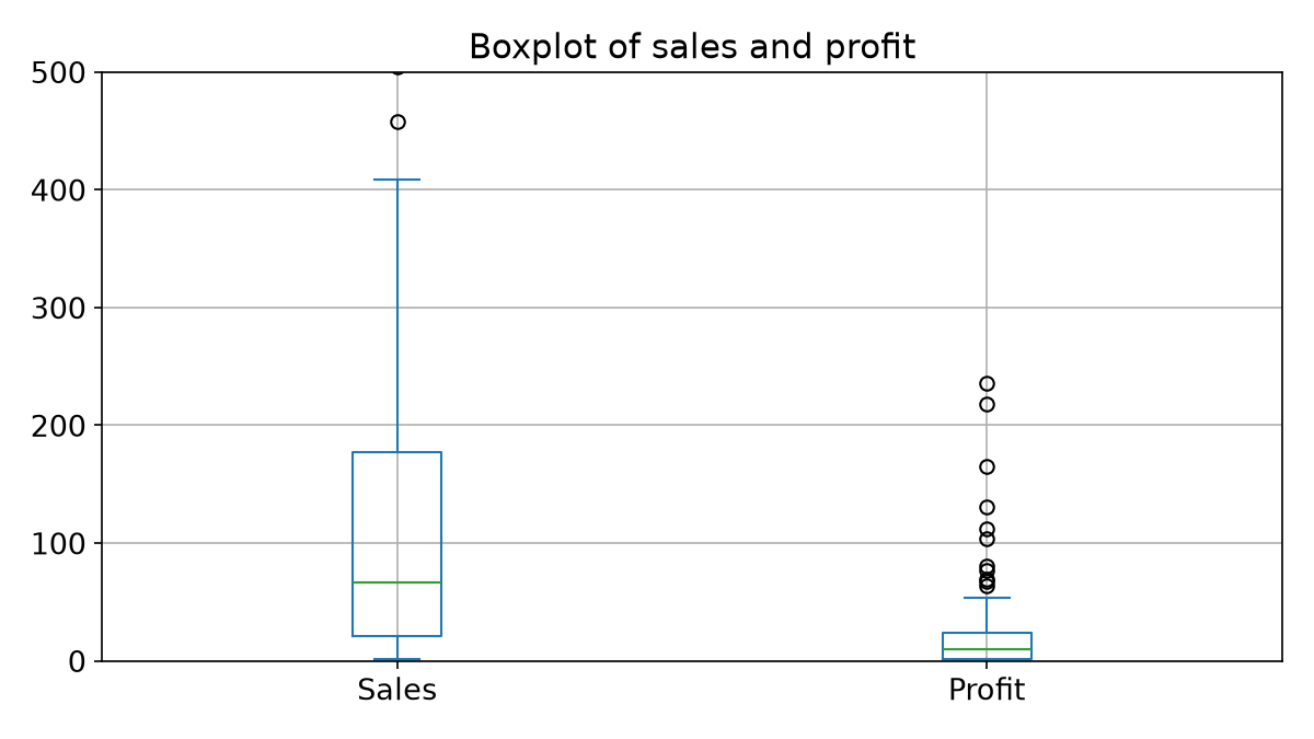
The box spans the middle half of the values and the line inside it is the median. plt.ylim(0, 500) zooms in on the boxes: 12 sales and 1 profit above 500, and the 20 negative profits, fall outside the chart.
unique and nunique
df['State'].nunique()       # 49
df['Country'].unique()      # ['United States']
df.drop('Country', axis=1, inplace=True)
df.shape                    # (9994, 19)
unique() lists the distinct values of a column and nunique() counts them. Country holds a single value in every row, so it carries no information and the notebook drops it.
Worked example: a boolean mask
The rest of this part uses the first 10 orders and three columns:
df_subset = df.loc[[i for i in range(10)], ['Ship Mode', 'State', 'Sales']] Ship Mode State Sales
0 Second Class Kentucky 261.9600
1 Second Class Kentucky 731.9400
2 Second Class California 14.6200
3 Standard Class Florida 957.5775
4 Standard Class Florida 22.3680
5 Standard Class California 48.8600
6 Standard Class California 7.2800
7 Standard Class California 907.1520
8 Standard Class California 18.5040
9 Standard Class California 114.9000Question. Which rows does df_subset[df_subset['Sales'] > 100] keep?
Answer. df_subset['Sales'] > 100 is a Series of True and False values, one per row: True for rows 0, 1, 3, 7 and 9. Putting it inside the brackets keeps exactly those rows, each with its own index label:
        Ship Mode       State     Sales
0    Second Class    Kentucky  261.9600
1    Second Class    Kentucky  731.9400
3  Standard Class     Florida  957.5775
7  Standard Class  California  907.1520
9  Standard Class  California  114.9000
Conditions combine with & (both must be true) and | (at least one is true), and each condition needs its own parentheses:
df_subset[(df_subset['State'] != 'California') & (df_subset['Sales'] > 100)]This keeps rows 0, 1 and 3; rows 7 and 9 are dropped because they are in California.
The notebook also runs df_subset > 100 on the whole DataFrame. In current pandas this raises TypeError: '>' not supported between instances of 'str' and 'int', because two of the three columns hold text. Build a mask from one column, as above.
Setting and resetting the index
The notebook builds a small DataFrame whose index is the letters A to E:
   Age  Height  Weight
A   22      66     140
B   42      70     148
C   30      62     125
D   35      68     160
E 25 62 152df1.reset_index()moves the letters into a column calledindexand numbers the rows from 0.df1.reset_index(drop=True)numbers the rows from 0 and throws the letters away.- After adding a column with
df1['Profession'] = "Student Teacher Engineer Doctor Nurse".split(),df1.set_index('Profession')makes that column the index, so.loc['Engineer']returns Age 30, Height 62, Weight 125.
groupby: split, apply, combine
df_subset.groupby('State') does three things:
- Split the rows into groups, one per state: California has 6 rows, Florida 2 and Kentucky 2.
- Apply an aggregate, such as the mean, to each group.
- Combine the answers into one row per group, sorted by the group label.
Worked example: mean sales per state
Question. Compute the mean Sales of each state from the 10 rows above.
Answer.
Florida:    (957.5775 + 22.368) / 2 = 489.97275
Kentucky:   (261.96 + 731.94) / 2  = 496.95
California: (14.62 + 48.86 + 7.28 + 907.152 + 18.504 + 114.9) / 6 = 1111.316 / 6 = 185.219333
pandas prints:
                 Sales
State
California  185.219333
Florida     489.972750
Kentucky    496.950000
groupby in current pandas
The notebook calls byState.mean() on the whole grouped DataFrame. In current pandas this raises a TypeError, because the Ship Mode column holds text that cannot be averaged, and byState.sum() does not fail but glues the Ship Mode text of each group together. Ask for the numeric columns only, or pick the column first:
byState = df_subset.groupby('State')
byState.mean(numeric_only=True)     # the table above
byState.sum(numeric_only=True)      # California 1111.3160, Florida 979.9455, Kentucky 993.9000
byState['Sales'].mean()             # the same means, as a Series
describe() works per group too. byState.describe() gives the count, mean, standard deviation, minimum, quartiles and maximum of Sales in each state; for California they are 6, 185.219333, 355.889307, 7.28, 15.591, 33.682, 98.39 and 907.152. Grouping by two columns, df.groupby(['State', 'City']) on the whole data makes 604 groups.
Open the DataFrame operations visualizer full screen to watch a boolean mask, groupby, pivot_table, apply, sort_values and merge work on these 10 orders one step at a time.
Part 3: Missing values, joins and reshaping
Find the missing values
The workbook's Missing sheet has 11 rows and 6 columns, with a few empty cells:
df_missing = pd.read_excel(url, sheet_name="Missing")
for c in df_missing.columns:
    miss = df_missing[c].isnull().sum()
    if miss > 0:
        print("{} has {} missing value(s)".format(c, miss))
    else:
        print("{} has NO missing value!".format(c))
Customer has 1 missing value(s)
Product has 2 missing value(s)
Sales has 1 missing value(s)
Quantity has 1 missing value(s)
Discount has NO missing value!
Profit has 1 missing value(s)isnull() returns a table of True and False of the same shape, and .sum() counts the True values in each column. The columns other than Customer look like this:
        Product     Sales  Quantity  Discount   Profit
0           NaN  1706.184       9.0       0.2  85.3092
1        Phones   911.424       4.0       0.2  68.3568
2           Art     8.560       2.0       0.0   2.4824
3        Phones       NaN       3.0       0.2  16.0110
4       Binders    22.720       4.0       0.2   7.3840
5       Binders    11.648       NaN       0.2   4.2224
6   Accessories    90.570       3.0       0.0  11.7741
7           NaN    77.880       2.0       0.0      NaN
8   Accessories    13.980       2.0       0.0   6.1512
9       Binders    25.824       6.0       0.2   9.3612
10        Paper   146.730       3.0       0.0  68.9631
The missing Customer value is in row 8.
Worked example: fill the missing sale
df_missing.fillna('FILL') writes the text FILL into every empty cell. For a number column you usually want a number. The Sales column is missing its value in row 3, between 8.560 in row 2 and 22.720 in row 4.
Question. What goes into row 3 with forward fill, with backward fill, and with the column mean?
Answer.
df_missing['Sales'].ffill()copies the value above: 8.56.df_missing['Sales'].bfill()copies the value below: 22.72.- The 10 known sales add up to 3015.52, so the mean is
3015.52 / 10 = 301.552, anddf_missing['Sales'].fillna(df_missing['Sales'].mean())puts 301.552 in row 3.
The notebook writes fillna(method='ffill') and fillna(df_missing.mean()['Sales']). The first raises TypeError in pandas 3 (pandas 2.2 still runs it with a warning), and the second fails in both versions because df_missing.mean() tries to average the text columns. Use .ffill(), .bfill() and the mean of the one column, as above.
Worked example: dropna
The non-null counts of the six columns are: Customer 10, Product 9, Sales 10, Quantity 10, Discount 11, Profit 10.
Question. What survives df_missing.dropna(axis=0), df_missing.dropna(axis=1) and df_missing.dropna(axis=1, thresh=10)?
Answer.
axis=0drops every row with at least one gap. The 6 complete rows survive: 1, 2, 4, 6, 9 and 10.axis=1drops every column with at least one gap. OnlyDiscount, the one full column, survives.thresh=10keeps the columns with at least 10 values, so onlyProduct, with 9, is dropped.
Spotting outliers with a boxplot
The notebook takes 50 random orders and plants two wrong sales, -1000 and -500, then draws the boxplot again:
df_sample = df[['Customer ID', 'State', 'Sales', 'Profit']].sample(n=50, random_state=1).copy()
df_sample.iloc[5, 2] = -1000.0
df_sample.iloc[15, 2] = -500.0
df_sample.plot.box()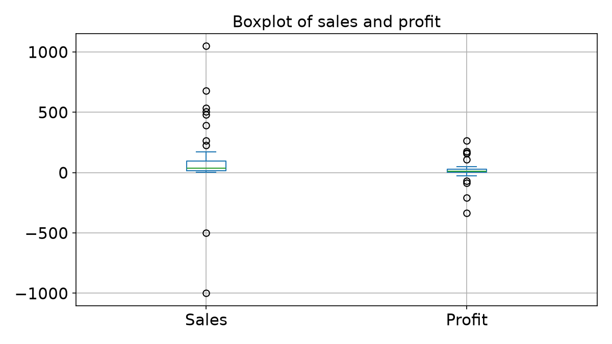
A sale can never be negative, so the two points far below the Sales box are the errors. We added random_state=1 so that the sample, and this figure, come out the same every time.
The notebook plants the values with df_sample['Sales'].iloc[5] = -1000.0. That is a chained assignment: the first bracket returns a separate Series and the value is written into it. In pandas 3 it changes nothing in df_sample (pandas 2.2 still changes it, with a warning). df_sample.iloc[5, 2], row position 5 and column position 2 (Sales), writes into the DataFrame itself.
Worked example: concat
Take three small tables of 2 orders each, with the columns Customer ID, State, Sales and Profit: a holds rows 0 and 1, b rows 2 and 3, and c rows 4 and 5. (The notebook takes three random samples of 4 orders; fixed rows give the same numbers every time.)
Question. What is the shape of pd.concat([a, b, c], axis=0), and of pd.concat([a, b, c], axis=1)?
Answer.
axis=0stacks the rows: shape(6, 4).axis=1puts the tables side by side and lines them up on the index: shape(6, 12). No row label appears in two tables, so each row has values in only one block of 4 columns, and 48 of the 72 cells areNaN.
Worked example: merge on a key
merge joins two tables on a common column, the key. The notebook merges on the customer's name; here we use Customer ID, which gives the same result:
df_1 = df[['Customer ID', 'Ship Date', 'Ship Mode']][0:4]
df_2 = df[['Customer ID', 'Sub-Category', 'Quantity']][0:4]
Both tables hold rows 0 to 3, whose keys are CG-12520, CG-12520, DV-13045 and SO-20335.
Question. How many rows does pd.merge(df_1, df_2, on='Customer ID', how='inner') have?
Answer. Every row on the left pairs with every row on the right that has the same key. CG-12520 is in 2 rows on each side, so it gives 2 × 2 = 4 rows; DV-13045 and SO-20335 give 1 row each. In total 4 + 1 + 1 = 6 rows:
  Customer ID  Ship Date       Ship Mode Sub-Category  Quantity
0    CG-12520 2016-11-11    Second Class    Bookcases         2
1    CG-12520 2016-11-11    Second Class       Chairs         3
2    CG-12520 2016-11-11    Second Class    Bookcases         2
3    CG-12520 2016-11-11    Second Class       Chairs         3
4    DV-13045 2016-06-16    Second Class       Labels         2
5    SO-20335 2015-10-18  Standard Class       Tables         5
Rows 2 and 3 repeat rows 0 and 1, because the two CG-12520 rows of df_1 are identical. .drop_duplicates() removes them and leaves 4 rows.
Inner, left, right and outer
Now merge df_1 with df_3 = df[['Customer ID', 'Sub-Category', 'Quantity']][2:6], whose keys are DV-13045, SO-20335, SO-20335 and BH-11710. The how option decides which keys survive:
| how | Keeps | Rows |
|---|---|---|
inner | the keys found in both tables | 3 |
left | every row of df_1 | 5 |
right | every row of df_3 | 4 |
outer | every key of both tables, sorted | 6, then 5 after drop_duplicates() |
The outer merge after drop_duplicates():
  Customer ID  Ship Date       Ship Mode Sub-Category  Quantity
0    BH-11710        NaT             NaN  Furnishings       7.0
1    CG-12520 2016-11-11    Second Class          NaN       NaN
3    DV-13045 2016-06-16    Second Class       Labels       2.0
4    SO-20335 2015-10-18  Standard Class       Tables       5.0
5    SO-20335 2015-10-18  Standard Class      Storage       2.0
A missing match is filled with NaN, and with NaT ("not a time") in a date column. Because Quantity now holds a NaN, it turned into a float column.
join does the same work on the index instead of a column. After df_1.set_index(['Customer ID'], inplace=True) and the same for df_3, df_1.join(df_3, how='outer').drop_duplicates() gives the same 5 rows, with Customer ID as the index.
sample and value_counts
df.sample(n=5)returns 5 random rows anddf.sample(frac=0.001)returns 0.1 percent of the rows, which is 10 of the 9994. Each run picks different rows unless you passrandom_state.df['Ship Mode'].value_counts()counts each distinct value: Standard Class 5968, Second Class 1945, First Class 1538, Same Day 543. The notebook runs it on the customer column to find the most frequent customers; byCustomer IDthe top one,WB-21850, has 37 order lines.
pivot_table
pivot_table groups by the index columns and applies aggfunc to the values columns:
df.pivot_table(values=['Sales', 'Quantity', 'Profit'], index=['Region'], aggfunc='mean')Rounded to 2 decimals:
| Region | Profit | Quantity | Sales |
|---|---|---|---|
| Central | 17.09 | 3.78 | 215.77 |
| East | 32.14 | 3.73 | 238.34 |
| South | 28.86 | 3.83 | 241.80 |
| West | 33.85 | 3.83 | 226.49 |
The notebook runs it on a random sample of 100 orders with index=['Region', 'State'], which makes one row per region and state pair. On the full data every number is the same each time you run it.
sort_values
df_subset.sort_values(by='Sales') orders the 10 rows from the smallest sale to the largest: row 6 (7.28) comes first and row 3 (957.5775) last, and each row keeps its index label. sort_values(by=['State', 'Sales']) sorts by State first and breaks ties by Sales, so the six California rows come first, from 7.28 to 907.152.
Worked example: apply a function
apply calls a function once for every value of a column and returns the answers as a new Series:
def categorize_sales(price):
    if price < 50:
        return "Low"
    elif price < 200:
        return "Medium"
    else:
        return "High"

df_subset['Sales Price Category'] = df_subset['Sales'].apply(categorize_sales)
Question. What does categorize_sales return for 261.96, 14.62 and 114.9?
Answer. 261.96 is not below 200, so High; 14.62 is below 50, so Low; 114.9 is not below 50 but is below 200, so Medium. On all 9994 orders the categories are Low 4849, High 2579 and Medium 2566.
A short function can be written in place with lambda. df_subset['Sales'].apply(lambda x: 0.85*x if x > 200 else x) gives 15 percent off every sale above 200: row 0 becomes 0.85 × 261.96 = 222.666, and row 2, 14.62, stays as it is. apply(len) on a text column returns the length of each value; on State it gives 8 for Kentucky and 10 for California.
Common mistakes
- A single column after reading: the
sepdoes not match the file. - Losing the first row: the file has no header line, so pass
header=None. nameswithoutheader=0on a file that has a header: the old header becomes a data row.- Reading a bare file name in Colab: the file is not there; use the repository address.
- Forgetting the parentheses around each condition joined by
&or|. - Running the notebook's older calls as they are:
fillna(method=...),mean()on a DataFrame with text columns, and chained assignment such asdf['Sales'].iloc[5] = value. - Merging on a key that repeats on both sides without checking how many rows came out.
Project milestone: form your team
This week's milestone starts the course project:
- Form a team of 3 members with a project idea, or a team of 2 members with a research paper.
- Write down the question your project answers, or the paper you will study.
- Find the dataset and load it with the reader that fits its format:
read_csv,read_excel,read_html,read_jsonor another from Part 1. - Right after loading, check its
shape, its column names andisnull().sum().
Next week the milestone is the project or paper proposal, and the lesson turns DataFrames into charts with Matplotlib and Seaborn.
Key takeaways
- pandas has one reader per format; each returns a DataFrame, except
read_htmlandread_pdf, which return a list of them, andread_excelwithsheet_name=None, which returns a dict. - Check the shape and the column names right after reading: they reveal a wrong
sep, a missing header or junk lines. - Filter rows with a boolean mask, and summarise groups with
groupbyandpivot_table. - Find gaps with
isnull, then decide whether to fill them or drop them. - Join tables with
concat,mergeorjoin, and count the rows of the result.
Practice
About 30 minutes. Try each task before you read its answer at the end of the page.
Practice 1: a messy export (about 5 minutes)
A lab system exported this file, p1_scores.txt:
Exported by the lab system
Section 3
ID;Name;Quiz;Lab
101;A1;7;9
102;B2;5;8
103;C3;9;10
104;D4;6;7
End of export- What shape does
pd.read_csv('p1_scores.txt')give with no options, and why? - Write the
read_csvcall that gives a clean table, and state its shape and column names. - Change your call to read only the first 2 students.
Practice 2: mask, groupby and apply (about 8 minutes)
  Region       Ship Mode  Sales
0   East     First Class  120.0
1   West  Standard Class   45.5
2   East  Standard Class  310.0
3  South    Second Class   80.0
4   West     First Class  220.0
5  South  Standard Class   15.0
6   East    Second Class   95.0
7 West Standard Class 60.5- Which rows does
df[(df['Sales'] > 100) & (df['Region'] != 'West')]keep? - Compute the sum and the mean of
Salesfor each region withgroupby('Region'). - Apply
categorize_salestoSales. How many orders fall in each category?
Practice 3: missing values (about 5 minutes)
A DataFrame has three columns and 5 rows:
Qty: 4, NaN, 6, NaN, 10Price: 2.5, 3.0, NaN, 4.0, 5.5Item: pen, ink, None, pad, tape
- Give
Qtyafterffill()and afterbfill(). - Give
Qtyafter filling with its own mean. - Which rows survive
dropna(axis=0)? Which columns survivedropna(axis=1, thresh=4)?
Practice 4: count the merge rows (about 5 minutes)
left:Key= K1, K2, K2, K3 andA= 1, 2, 3, 4right:Key= K2, K3, K3, K4 andB= 10, 20, 30, 40
How many rows does pd.merge(left, right, on='Key', how=...) return for how = 'inner', 'left', 'right' and 'outer'? Explain each count before you run it.
Practice 5: in Colab, on the superstore data (about 7 minutes)
Load the superstore orders as in Part 2, then:
- How many orders come from Texas?
- Compute the total
SalesandProfitof eachCategorywithgroupby. - How many orders lost money (
Profitbelow 0)? - Use
pivot_tablewithaggfunc='sum'to get the totalProfitof eachRegion. Which region is the lowest?
Answers
Answer 1
- With no options the shape is
(7, 1). The first line,Exported by the lab system, becomes the header, and since the file uses semicolons, not commas, every other line stays in one piece. - Skip the 2 lines at the top and the 1 at the bottom, and set the separator:
pd.read_csv('p1_scores.txt', sep=';', skiprows=2, skipfooter=1, engine='python') ID Name Quiz Lab
0 101 A1 7 9
1 102 B2 5 8
2 103 C3 9 10
3 104 D4 6 7The shape is (4, 4) and the columns are ID, Name, Quiz and Lab.
pd.read_csv('p1_scores.txt', sep=';', skiprows=2, nrows=2)reads students 101 and 102. Dropskipfooterhere: pandas refuses to combine it withnrows(ValueError: 'skipfooter' not supported with 'nrows'), and withnrows=2the footer is never reached anyway.
Answer 2
- Rows 0 and 2. Rows 0, 2 and 4 have sales above 100, and row 4 is in the West.
- Sums: East
120 + 310 + 95 = 525.0, South80 + 15 = 95.0, West45.5 + 220 + 60.5 = 326.0. Means: East525 / 3 = 175.0, South95 / 2 = 47.5, West326 / 3 = 108.666667. - The categories in row order are Medium, Low, High, Medium, High, Low, Medium, Medium, so Medium 4, Low 2 and High 2.
Answer 3
ffill(): 4, 4, 6, 6, 10.bfill(): 4, 6, 6, 10, 10.- The mean of the known values is
(4 + 6 + 10) / 3 = 6.666667, soQtybecomes 4, 6.666667, 6, 6.666667, 10. - Only rows 0 and 4 have no gap. With
thresh=4,Price(4 values) andItem(4 values) survive, andQty(3 values) is dropped.
Answer 4
| how | Rows | Why |
|---|---|---|
inner | 4 | K2: 2 rows on the left × 1 on the right = 2; K3: 1 × 2 = 2 |
left | 5 | the 4 inner rows, plus K1 with B = NaN |
right | 5 | the 4 inner rows, plus K4 with A = NaN |
outer | 6 | the 4 inner rows, plus K1 and K4 |
Answer 5
df[df['State'] == 'Texas'].shapeis(985, 19): 985 orders.df.groupby('Category')[['Sales', 'Profit']].sum():
| Category | Sales | Profit |
|---|---|---|
| Furniture | 741999.7953 | 18451.2728 |
| Office Supplies | 719047.0320 | 122490.8008 |
| Technology | 836154.0330 | 145454.9481 |
Furniture sells about as much as the other two categories but earns far less profit.
(df['Profit'] < 0).sum()is 1871 orders.df.pivot_table(values=['Profit'], index=['Region'], aggfunc='sum')gives Central 39706.3625, East 91522.7800, South 46749.4303 and West 108418.4489. The lowest is Central.