

Decision Trees and Random Forest
This section introduces two classifiers that make predictions by asking questions. A decision tree asks a short chain of yes or no questions about a sample, such as "is the credit score at most 677?", and reads the answer at the end of the chain. A random forest grows many different trees and lets them vote. You will first grow a small tree by hand on ten real borrowers, then train a tree and a forest in scikit-learn on the Lending Club loans of week 6.
Objectives
By the end of the section you should be able to:
- Explain how a decision tree classifies a sample: a chain of threshold questions that ends in a leaf.
- Compute the Gini impurity of a node and the weighted Gini of a split by hand, and use it to choose a split.
- Explain why a tree grown until every leaf is pure fits the training data perfectly but predicts new data poorly.
- Explain the three ideas of a random forest: bootstrap samples, a random subset of features at each split, and a majority vote.
- Train
DecisionTreeClassifierandRandomForestClassifieron the Lending Club data and read their confusion matrices. - Recognise when a high accuracy only reflects an unbalanced target, and apply the same steps to your team project.
Where this sits in the course
Week 6 of the plan has three parts:
- One notebook.
DecisionTrees_RandomForest_Classificationtrains a decision tree and a random forest on public lending data. - A real-world scenario. Lending Club connects people who need money (borrowers) with people who have money (investors). We try to create a model to predict the risk of lending money to someone given a wide range of credit related data: we predict whether or not the borrower paid back their loan in full.
- A project milestone. Machine Learning Model Implementation: your team keeps implementing models on its own data.
In week 5 you classified with KNN, which measures distances. A tree measures no distance at all: it only compares one feature with one threshold at a time. The fit, predict and score pattern stays exactly the same.
| Part | What we do | Time |
|---|---|---|
| 1 | The idea of a tree, and a tree grown by hand | 30 min |
| 2 | The Lending Club notebook: data and exploration | 15 min |
| 3 | One decision tree on the loans | 10 min |
| 4 | Random forest: by hand, then on the loans | 25 min |
| 5 | Mistakes, project, practice with answers, takeaways | 40 min |
Part 1: The idea of a decision tree
What a decision tree is
A decision tree classifies a sample by asking a sequence of questions about its features. Each question compares one feature with a threshold, for example fico ≤ 677. The answer sends the sample down the left branch (yes) or the right branch (no), where the next question waits. When no question is left, the sample has reached a leaf, and the leaf's class is the prediction.
The vocabulary, on the loans
| Term | In the Lending Club data |
|---|---|
Features X | credit data of a borrower, such as fico (credit score) and int.rate (interest rate) |
Label y | not.fully.paid: 1 did not pay back in full, 0 paid in full |
| Root node | the first question, asked of every borrower |
| Internal node | a later question, asked only of the borrowers who reached it |
| Leaf | a node with no question; it predicts the majority class of its training borrowers |
| Depth | the number of questions on the longest path from the root to a leaf |
How a tree chooses a question: Gini impurity
A good question separates the classes: after it, each side should hold mostly one class. The notebook builds its tree with criterion='gini', which measures how mixed a node is with the Gini impurity:
G = 1 - (p0^2 + p1^2)Here p0 is the fraction of the node's borrowers in class 0 (paid) and p1 the fraction in class 1 (not paid). Two cases fix the scale:
- A pure node, all one class:
p0 = 1,p1 = 0, soG = 1 - 1 = 0. - A 50 to 50 node:
G = 1 - (0.25 + 0.25) = 0.5, the largest value two classes can reach.
A question splits a node of n borrowers into a left side of nL and a right side of nR. The quality of the question is the weighted Gini of the two sides, where each side counts in proportion to its size:
Gw = (nL / n) * GL + (nR / n) * GRGL and GR are the Gini impurities of the left and right sides. The tree tries every feature and every threshold, and keeps the question with the lowest Gw, which is the same as the largest decrease G - Gw. The candidate thresholds are the midpoints between neighbouring values of the feature in the node.
Worked example: a tree grown by hand
We take ten real borrowers from the Lending Club data and use two features, fico and int.rate. Four of them did not pay back in full.
| Borrower | fico | int.rate | not.fully.paid |
|---|---|---|---|
| B1 | 647 | 0.1482 | 1 (not paid) |
| B2 | 662 | 0.1507 | 0 (paid) |
| B3 | 667 | 0.1299 | 1 (not paid) |
| B4 | 672 | 0.1347 | 1 (not paid) |
| B5 | 682 | 0.1103 | 0 (paid) |
| B6 | 687 | 0.1387 | 0 (paid) |
| B7 | 692 | 0.1284 | 0 (paid) |
| B8 | 707 | 0.1091 | 1 (not paid) |
| B9 | 727 | 0.1059 | 0 (paid) |
| B10 | 757 | 0.1189 | 0 (paid) |
These are rows 8443, 1259, 380, 1794, 520, 1183, 2472, 142, 7764 and 2217 of loan_data.csv, sorted by fico.
Step 1: the Gini of the root
The root holds all ten borrowers: 6 paid and 4 not paid.
G = 1 - (0.6^2 + 0.4^2) = 1 - (0.36 + 0.16) = 0.48The root is close to the worst value, 0.5: the two classes are well mixed.
Step 2: try the question fico ≤ 677
677 is the midpoint between B4 (672) and B5 (682). The question sends B1 to B4 to the left and B5 to B10 to the right.
- Left, 4 borrowers: B1, B3 and B4 not paid, B2 paid. So 3 not paid, 1 paid.
- Right, 6 borrowers: only B8 not paid. So 1 not paid, 5 paid.
Step 3: the Gini of each side
GL = 1 - ((3/4)^2 + (1/4)^2) = 1 - (0.5625 + 0.0625) = 0.375
GR = 1 - ((1/6)^2 + (5/6)^2) = 1 - (1/36 + 25/36) = 10/36 = 0.2778
Both sides are purer than the root (0.48).
Step 4: the weighted Gini of the split
Gw = (4/10) * 0.375 + (6/10) * 0.2778 = 0.15 + 0.1667 = 0.3167The decrease is 0.48 - 0.3167 = 0.1633.
Step 5: the other feature
The best question on int.rate is int.rate ≤ 0.12915, the midpoint between B3 (0.1299) and B7 (0.1284).
- Left, 5 borrowers with the lower rates: B5, B7, B8, B9, B10. Only B8 is not paid:
GL = 1 - (0.2^2 + 0.8^2) = 0.32. - Right, 5 borrowers with the higher rates: B1, B2, B3, B4, B6. Three are not paid:
GR = 1 - (0.6^2 + 0.4^2) = 0.48.
Gw = (5/10) * 0.32 + (5/10) * 0.48 = 0.400.40 is higher than 0.3167, so the credit score gives the better first question.
Step 6: the search tries every threshold
The ten fico values give nine midpoints. Their weighted Gini values:
| Threshold | Left: not paid, paid | Right: not paid, paid | Weighted Gini |
|---|---|---|---|
| 654.5 | 1, 0 | 3, 6 | 0.4000 |
| 664.5 | 1, 1 | 3, 5 | 0.4750 |
| 669.5 | 2, 1 | 2, 5 | 0.4190 |
| 677 | 3, 1 | 1, 5 | 0.3167 |
| 684.5 | 3, 2 | 1, 4 | 0.4000 |
| 689.5 | 3, 3 | 1, 3 | 0.4500 |
| 699.5 | 3, 4 | 1, 2 | 0.4762 |
| 717 | 4, 4 | 0, 2 | 0.4000 |
| 742 | 4, 5 | 0, 1 | 0.4444 |
The nine int.rate midpoints give values between 0.40 and 0.4762. So the lowest of all eighteen candidates is fico ≤ 677, and it becomes the root question.
Step 7: grow the left child
The left child holds B1 to B4 (3 not paid, 1 paid, G = 0.375). The paid borrower B2 has the highest rate of the four (0.1507), so int.rate ≤ 0.14945 separates it:
- Left: B1, B3, B4, all not paid,
G = 0. - Right: B2, paid,
G = 0.
The weighted Gini is 0: both sides are pure and become leaves. (The best fico question here, fico ≤ 664.5, only reaches 0.25.)
Step 8: grow the right child
The right child holds B5 to B10 (1 not paid, 5 paid, G = 0.2778). The only defaulter, B8, has a good score (707) and a low rate (0.1091). The best question is int.rate ≤ 0.1097:
- Left: B9 and B8, 1 paid and 1 not paid,
G = 0.5. - Right: B5, B6, B7, B10, all paid,
G = 0.
Gw = (2/6) * 0.5 + (4/6) * 0 = 0.1667The best fico question for this node, fico ≤ 699.5, gives 0.2222, so the rate wins again.
The tree we built
fico <= 677 ?
|-- yes: int.rate <= 0.14945 ?
|        |-- yes: leaf [3 not paid, 0 paid]  -> not paid
|        |-- no:  leaf [0 not paid, 1 paid]  -> paid
|-- no:  int.rate <= 0.1097 ?
         |-- yes: leaf [1 not paid, 1 paid]  -> paid (a tie goes to class 0)
         |-- no:  leaf [0 not paid, 4 paid]  -> paid
scikit-learn builds exactly this tree from the same ten rows with DecisionTreeClassifier(max_depth=2): the same questions, the same thresholds and the same Gini values (0.48 at the root, 0.375 and 0.2778 at the two children). When a leaf holds a tie, scikit-learn predicts the class with the smaller number, here 0.
Predict two new borrowers
- fico 670, int.rate 0.14. 670 ≤ 677, so go left. 0.14 ≤ 0.14945, so go left again. The leaf predicts not paid.
- fico 700, int.rate 0.12. 700 > 677, so go right. 0.12 > 0.1097, so go right again. The leaf predicts paid.
Open the decision tree builder full screen to grow this tree yourself. Choose a feature, move the threshold and watch the Gini values, or press Play to watch the search try every threshold, then Split.
Entropy, the notebook's other criterion
The notebook also trains forests with criterion='entropy', a second measure of how mixed a node is:
H = -(p0 * log2(p0) + p1 * log2(p1))A pure node has H = 0 and a 50 to 50 node has H = 1. For our root, H = -(0.6 * log2(0.6) + 0.4 * log2(0.4)) = 0.971. With entropy, scikit-learn picks the same first question here, fico ≤ 677. The two criteria usually agree on which splits are good.
A tree that never stops
The notebook grows its tree with max_depth=None: the tree keeps splitting until every leaf is pure. On our ten borrowers, one more question, fico ≤ 717, separates B8 from B9. The full tree has depth 3 and 5 leaves, and it classifies all ten training borrowers correctly. That last question exists only to isolate one borrower. A tree that grows until it memorises its training rows is overfitting: it learns the accidents of the training set, and new borrowers pay the price. Part 3 shows this on the real data.
Part 2: The Lending Club notebook
Open the notebook
Open DecisionTrees_RandomForest_Classification in Colab
The notebook reads loan_data.csv from its own folder. In Colab that file is not there: in the repository it lives in the Datasets folder. Read it from the repository instead:
import pandas as pd
import numpy as np
import matplotlib.pyplot as plt
import seaborn as sns

url = ("https://raw.githubusercontent.com/"
       "tirthajyoti/Machine-Learning-with-Python/"
       "master/Datasets/loan_data.csv")
df = pd.read_csv(url)
df.info()
Load and inspect the data
df.info() reports 9578 rows and 14 columns, with no missing values. The columns the notebook describes include:
| Column | Meaning |
|---|---|
credit.policy | 1 if the borrower meets the credit underwriting criteria of LendingClub.com, 0 otherwise |
purpose | the purpose of the loan, text such as credit_card or debt_consolidation |
int.rate | the interest rate as a proportion (11% is stored as 0.11); riskier borrowers get higher rates |
fico | the FICO credit score of the borrower |
not.fully.paid | the label: 1 if the borrower did not pay back in full |
The other eight columns are numbers too: the monthly installment, the log of the annual income, the debt-to-income ratio, the days with a credit line, the revolving balance and utilisation, the inquiries in the last 6 months, the late payments in 2 years and the public records.
The two counts that matter
print(df['credit.policy'].value_counts())
print(df['not.fully.paid'].value_counts())credit.policy: 7710 borrowers meet the criteria, 1868 do not.not.fully.paid: 8045 paid in full and 1533 did not. Only 16% of the borrowers are in class 1.
Keep the second count in mind. A model that answers "paid" for everybody is already right 84% of the time.
Explore before you model
The notebook draws a histogram of fico for each value of credit.policy:
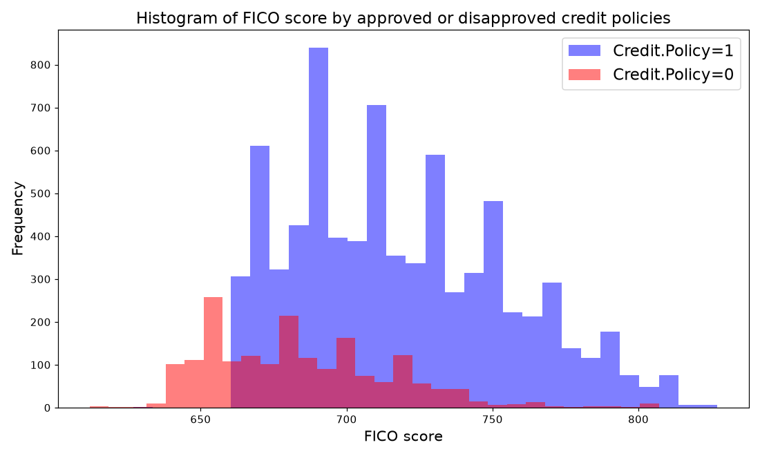
Almost every borrower with a score below 660 fails the credit policy: 487 borrowers against 2. A single threshold on one feature separates a group well, which is exactly the kind of question a tree asks.
It then counts the loans by purpose, coloured by not.fully.paid:
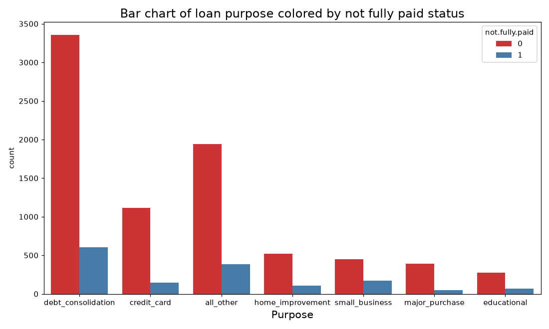
debt_consolidation is the most common purpose (3957 loans). The share not paid in full varies by purpose: 27.8% for small_business, 11.6% for credit_card and 11.2% for major_purchase.
The later lmplot cell passes size=6. Current versions of seaborn renamed that argument, and the cell stops with TypeError: lmplot() got an unexpected keyword argument 'size'. Write height=6 instead.
Turn the text column into numbers
purpose holds text, and scikit-learn needs numbers. The notebook creates dummy variables:
df_final = pd.get_dummies(df, ['purpose'], drop_first=True)- The seven purposes become six 0 or 1 columns, such as
purpose_credit_card.drop_first=Truedrops the first purpose,all_other: a borrower with 0 in all six columns has that purpose. df_finalhas 19 columns: the 12 other feature columns, the 6 dummies and the label.- The second argument here is the
prefixof the new columns. The clearer form ispd.get_dummies(df, columns=['purpose'], drop_first=True), which gives the same 19 columns.
Split into training and test sets
from sklearn.model_selection import train_test_split

X = df_final.drop('not.fully.paid', axis=1)
y = df_final['not.fully.paid']
X_train, X_test, y_train, y_test = train_test_split(
X, y, test_size=0.30, random_state=101)Xhas 18 feature columns.test_size=0.30keeps 2874 borrowers for testing and trains on 6704.- The test set holds 2431 borrowers who paid and 443 who did not.
- The notebook calls
train_test_splitwithoutrandom_state, so every run gives a different split and slightly different numbers. We addrandom_state=101so that your numbers match this page.
Part 3: One decision tree on the loans
Fit and predict
from sklearn.tree import DecisionTreeClassifier

dtree = DecisionTreeClassifier(criterion='gini', max_depth=None,
                               random_state=101)
dtree.fit(X_train, y_train)
predictions = dtree.predict(X_test)
criterion='gini' is the impurity of Part 1. max_depth=None lets the tree grow until every leaf is pure. random_state=101 fixes the order in which features are tried, so ties between equally good splits are broken the same way on every run.
Worked example: evaluate the tree
from sklearn.metrics import classification_report, confusion_matrix

cm = confusion_matrix(y_test, predictions)
print(cm)
print("Accuracy of prediction:", round((cm[0,0]+cm[1,1])/cm.sum(), 3))| Predicted 0 (paid) | Predicted 1 (not paid) | |
|---|---|---|
| Actual 0 (paid) | 1975 | 456 |
| Actual 1 (not paid) | 336 | 107 |
- Correct:
1975 + 107 = 2082of 2874, so the accuracy is2082 / 2874 = 0.724. The notebook printsAccuracy of prediction: 0.724. - Recall of class 1: of the 443 borrowers who did not pay, the tree found
107 / 443 = 0.24. - Precision of class 1: of the
456 + 107 = 563borrowers the tree flagged,107 / 563 = 0.19really did not pay.
classification_report(y_test, predictions) prints the same values, rounded:
              precision    recall  f1-score   support

           0       0.85      0.81      0.83      2431
           1       0.19      0.24      0.21       443

    accuracy                           0.72      2874
   macro avg       0.52      0.53      0.52      2874
weighted avg       0.75      0.72      0.74      2874
The tree memorised its training set
print(dtree.get_depth(), dtree.get_n_leaves())
print(dtree.score(X_train, y_train))
The output is 27, 1005 and 1.0. The tree asks up to 27 questions, ends in 1005 leaves, and classifies every one of the 6704 training borrowers correctly. On the test borrowers it scores 0.724, lower than the 0.846 of answering "paid" for everyone. This is the overfitting of Part 1 at full size.
Part 4: Random forest
The idea: many different trees, one vote
A random forest trains many trees and combines their answers. Three ideas make the trees different from each other:
- A bootstrap sample for each tree. From the n training rows, draw n rows at random with replacement. Some rows are drawn twice or more, and others are left out. This is
bootstrap=Truein the fitted model. - A random subset of features at each split. At every node a tree searches only a few features chosen at random. With
max_features='sqrt', the default, it searchesmfeatures out ofp, wheremis the square root ofprounded down. - A vote. Every tree classifies the new sample. The class with the most votes wins. (scikit-learn averages the trees' class probabilities; when every leaf is pure, as in fully grown trees, that is exactly a count of votes.)
One deep tree changes a lot when a few training rows change. Many trees that each saw a different sample make different mistakes, and a vote cancels many of them.
Worked example: five trees on the ten borrowers
We fit RandomForestClassifier(n_estimators=5, random_state=0) on the ten borrowers of Part 1 and read each tree's bootstrap sample from rf.estimators_samples_. With p = 2 features, m = 1: every split searches a single random feature.
Tree 1 drew B4, B3, B1, B1, B3, B7, B10, B8, B4, B10. So B1, B3, B4 and B10 were drawn twice, B7 and B8 once, and B2, B5, B6 and B9 not at all. Its root question is fico ≤ 682, not 677: B5 (682) is not in its sample, so the midpoint falls between B4 (672) and B7 (692).
The new borrower has fico 710 and int.rate 0.11. Each tree votes:
| Tree | Borrowers left out of its sample | Vote |
|---|---|---|
| 1 | B2, B5, B6, B9 | not paid |
| 2 | B3, B6, B7 | paid |
| 3 | B1, B3, B7, B10 | paid |
| 4 | B2, B3, B7, B8, B10 | paid |
| 5 | B1, B3, B5, B9 | not paid |
The vote is 3 paid against 2 not paid, so the forest predicts paid. rf.predict_proba returns [0.6, 0.4]: 3 of 5 trees for class 0 and 2 of 5 for class 1. Trees 1 and 5 place the new borrower in a small region they built around B8, the defaulter with a good score nearby. The other three trees place it with the paid borrowers, and they outvote the first two.
Open the random forest vote widget full screen. Press Play to watch each tree draw its bootstrap sample and vote, drag the star to move the new borrower, or grow a new random forest of nine trees.
How many features at each split, on the loans
X_train has p = 18 features. The square root of 18 is 4.24, so each split searches 4 features chosen at random. The fitted forest confirms it: rfc.estimators_[0].max_features_ is 4.
A bootstrap sample leaves many rows out. Over the 600 trees below, each tree saw between 4160 and 4310 distinct borrowers of the 6704 training rows, 63.2% on average; the rest were never drawn for that tree.
Fit the forest
from sklearn.ensemble import RandomForestClassifier

rfc = RandomForestClassifier(n_estimators=600, random_state=101)
rfc.fit(X_train, y_train)
rfc_pred = rfc.predict(X_test)
print(confusion_matrix(y_test, rfc_pred))
print(classification_report(y_test, rfc_pred))
n_estimators=600 grows 600 trees. The notebook's printout of the fitted model shows the older default max_features='auto'; current scikit-learn calls the same setting 'sqrt'.
Worked example: the forest's confusion matrix
| Predicted 0 (paid) | Predicted 1 (not paid) | |
|---|---|---|
| Actual 0 (paid) | 2420 | 11 |
| Actual 1 (not paid) | 431 | 12 |
- Accuracy:
(2420 + 12) / 2874 = 0.846, much higher than the single tree's 0.724. - But the forest flags only
11 + 12 = 23of the 2874 test borrowers as not paid. Of the 443 who did not pay, it finds 12: recall12 / 443 = 0.03. - Answering "paid" for every borrower gives
2431 / 2874 = 0.846too. The forest beats that by a single borrower.
              precision    recall  f1-score   support

           0       0.85      1.00      0.92      2431
           1       0.52      0.03      0.05       443

    accuracy                           0.85      2874
   macro avg       0.69      0.51      0.48      2874
weighted avg       0.80      0.85      0.78      2874
The notebook asks at this point: "Do you get anything strange?" This is the strange part. With only 16% defaulters, most trees vote "paid" for almost everyone: no test borrower gets more than 375 of the 600 trees (62.5%) voting "not paid". A high accuracy on an unbalanced target can hide a model that rarely finds the class you care about. Always read the recall of that class, not only the accuracy.
A slip in the notebook
The notebook's cell for the forest's report is:
cr = classification_report(y_test, predictions)predictions holds the single tree's predictions, so that cell prints the tree's report a second time. Use rfc_pred, as in the code above.
How many trees?
The notebook trains forests of 5, 10, 15 and up to 100 trees, and records the accuracy of each:
nsimu = 21
accuracy = [0] * nsimu
ntree = [0] * nsimu
for i in range(1, nsimu):
    rfc = RandomForestClassifier(n_estimators=i*5, min_samples_split=10,
                                 max_depth=None, criterion='gini',
                                 random_state=101)
    rfc.fit(X_train, y_train)
    rfc_pred = rfc.predict(X_test)
    cm = confusion_matrix(y_test, rfc_pred)
    accuracy[i] = (cm[0,0] + cm[1,1]) / cm.sum()
    ntree[i] = i * 5
min_samples_split=10 stops splitting a node that holds fewer than 10 training rows. We add random_state=101 to each forest so that the loop gives the same numbers on every run.
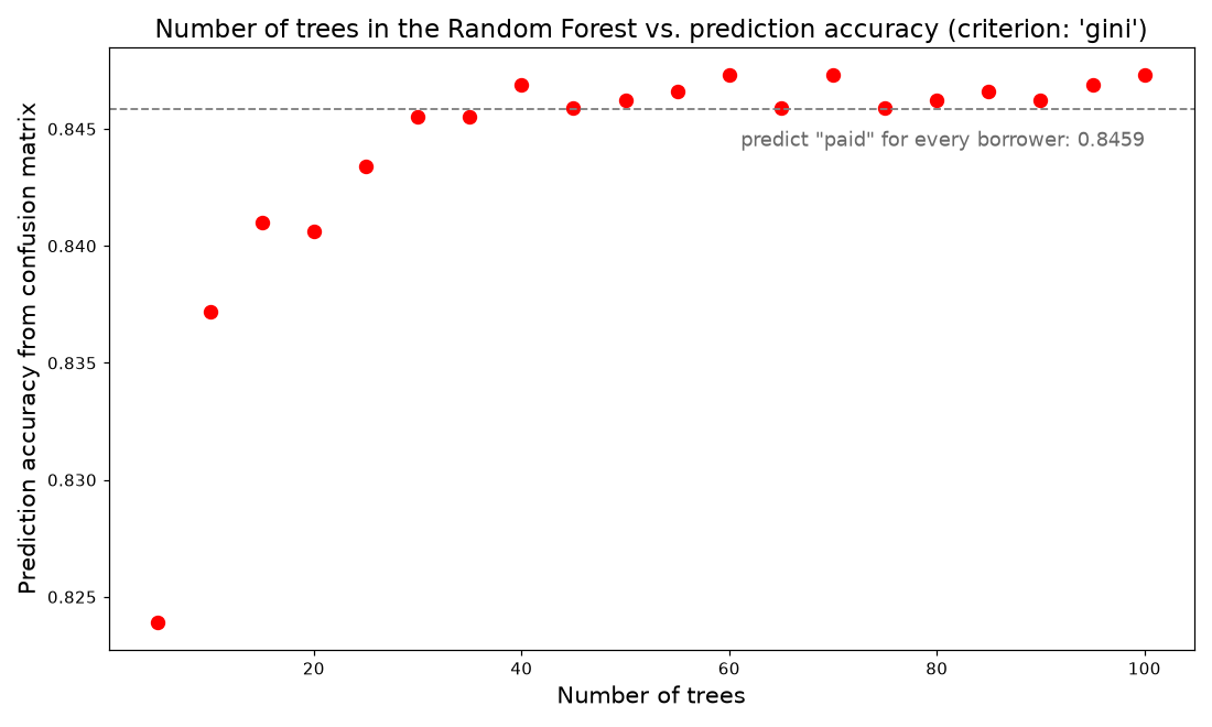
- With 5 trees the accuracy is 0.8239. It rises quickly and, from about 30 trees on, stays between 0.8455 and 0.8473.
- More trees make the vote steadier, but they cannot beat the limit of the data: the curve settles at the level of answering "paid" for everyone.
The notebook repeats the loop with other settings. The range of accuracies over the 20 forests of each run:
| Setting changed | Lowest accuracy | Highest accuracy |
|---|---|---|
none (gini, min_samples_split=10) | 0.8239 | 0.8473 |
criterion='entropy' | 0.8250 | 0.8473 |
max_depth=5 | 0.8434 | 0.8459 |
min_samples_split=2 | 0.8062 | 0.8466 |
min_samples_split=20 | 0.8302 | 0.8466 |
The differences at the top are one or two test borrowers out of 2874. Changing these settings does not fix the real problem, which is that the forest almost never predicts class 1.
Common mistakes
- Reading
loan_data.csvin Colab from a folder that does not contain it. - Forgetting
random_state, then comparing numbers from two different random splits. - Growing a tree with
max_depth=Noneand trusting its perfect training score. - Judging a model by accuracy alone when one class is rare.
- Printing the report of
predictionswhen you meantrfc_pred. - Passing a text column such as
purposeto scikit-learn without dummy variables.
Project milestone: model implementation
This week the milestone continues: implement a decision tree and a random forest on your team's project data.
- Take the features and the target you used for KNN last week. Convert any text column with
pd.get_dummies. - Split into a training set and a test set with a fixed
random_state. - Fit
DecisionTreeClassifierand compare its training score with its test score. - Fit
RandomForestClassifierand report its confusion matrix andclassification_report. - Compare the tree, the forest and last week's KNN on the same test set, and look at the recall of every class, not only the accuracy.
Key takeaways
- A decision tree classifies by a chain of threshold questions; a leaf predicts the majority class of its training rows.
- The tree chooses each question by the lowest weighted Gini impurity over every feature and threshold.
- A tree grown until every leaf is pure memorises its training set and overfits.
- A random forest trains many trees on bootstrap samples, with a random subset of features at each split, and takes a vote.
- When one class is rare, a high accuracy can hide a model that almost never finds that class: read the recall.
Practice
About 30 minutes. Try each task before you read its answer at the end of the page.
Practice 1: choose the first question (about 10 minutes)
Eight other real borrowers from loan_data.csv:
| Borrower | fico | int.rate | not.fully.paid |
|---|---|---|---|
| P1 | 647 | 0.1482 | 1 |
| P2 | 667 | 0.1343 | 0 |
| P3 | 677 | 0.1734 | 1 |
| P4 | 682 | 0.1197 | 0 |
| P5 | 692 | 0.1287 | 0 |
| P6 | 697 | 0.1316 | 1 |
| P7 | 742 | 0.1114 | 0 |
| P8 | 747 | 0.0751 | 0 |
- Compute the Gini impurity of the root.
- Compute the weighted Gini of the question
fico ≤ 679.5. - Compute the weighted Gini of the question
int.rate ≤ 0.13015. - Which question does the tree choose, and what is the decrease in Gini?
Practice 2: read the forest's confusion matrix (about 5 minutes)
Use the matrix of the 600-tree forest from Part 4: [[2420, 11], [431, 12]].
- Compute the precision and the recall of class 1.
- A "model" answers 0 (paid) for every test borrower. Write its confusion matrix and its accuracy.
- Which of the two models finds more of the borrowers who did not pay?
Practice 3: entropy of the first split (about 5 minutes)
For the ten borrowers of the worked example and the question fico ≤ 677, compute the entropy of the left side (3 not paid, 1 paid), the entropy of the right side (1 not paid, 5 paid), and their weighted entropy. The root entropy is 0.971.
Practice 4: in Colab, on the loans (about 10 minutes)
- Run the notebook up to the split, with
random_state=101and the data URL above. - Fit
DecisionTreeClassifier(max_depth=5, random_state=101). Print its confusion matrix, its test accuracy and its training accuracy. - Compare them with the tree grown with
max_depth=Nonein Part 3. - Rerun the loop over the number of trees with
max_depth=5. What range of accuracies do you get?
Answers
Answer 1
- The root holds 3 not paid and 5 paid:
G = 1 - ((3/8)^2 + (5/8)^2) = 1 - (9/64 + 25/64) = 30/64 = 0.4688. fico ≤ 679.5sends P1, P2, P3 to the left (2 not paid, 1 paid) and P4 to P8 to the right (1 not paid, P6, and 4 paid).GL = 1 - ((2/3)^2 + (1/3)^2) = 4/9 = 0.4444GR = 1 - ((1/5)^2 + (4/5)^2) = 8/25 = 0.32Gw = (3/8) * 0.4444 + (5/8) * 0.32 = 0.1667 + 0.2 = 0.3667
int.rate ≤ 0.13015sends P4, P5, P7, P8 to the left (all paid) and P1, P2, P3, P6 to the right (3 not paid, 1 paid).GL = 0GR = 1 - ((3/4)^2 + (1/4)^2) = 0.375Gw = (4/8) * 0 + (4/8) * 0.375 = 0.1875
- The tree chooses
int.rate ≤ 0.13015, because 0.1875 is lower than 0.3667. The decrease is0.4688 - 0.1875 = 0.2813. It is also the best of all 14 candidate thresholds, andDecisionTreeClassifier(max_depth=1)fitted on these eight rows asks exactly this question, with Gini values 0.46875, 0 and 0.375.
This time the interest rate wins: which feature is best depends on the rows in the node.
Answer 2
- Precision of class 1:
12 / (11 + 12) = 12 / 23 = 0.52. Recall of class 1:12 / (431 + 12) = 12 / 443 = 0.03. - Answering "paid" for everyone gives:
| Predicted 0 | Predicted 1 | |
|---|---|---|
| Actual 0 | 2431 | 0 |
| Actual 1 | 443 | 0 |
Its accuracy is 2431 / 2874 = 0.8459, against 2432 / 2874 = 0.8462 for the forest.
3. The forest finds 12 of the 443, the constant answer finds none. The accuracies differ by one borrower, and both models are nearly useless for finding defaulters.
Answer 3
- Left,
p1 = 3/4andp0 = 1/4:H = -(0.75 * log2(0.75) + 0.25 * log2(0.25)) = 0.3113 + 0.5 = 0.8113. - Right,
p1 = 1/6andp0 = 5/6:H = -((1/6) * log2(1/6) + (5/6) * log2(5/6)) = 0.4308 + 0.2192 = 0.6500. - Weighted:
(4/10) * 0.8113 + (6/10) * 0.6500 = 0.3245 + 0.3900 = 0.7145. The decrease from the root is0.971 - 0.7145 = 0.2565.
scikit-learn with criterion='entropy' reports the same three impurities for this split: 0.971, 0.8113 and 0.65.
Answer 4
- The tree with
max_depth=5:
| Predicted 0 | Predicted 1 | |
|---|---|---|
| Actual 0 | 2396 | 35 |
| Actual 1 | 431 | 12 |
- Test accuracy
(2396 + 12) / 2874 = 0.8379; training accuracy 0.845. - The unlimited tree scored 1.0 on training and 0.724 on test. Limiting the depth closes the gap between the two scores: the shallow tree no longer memorises the training borrowers. It finds only 12 of the 443 defaulters, though, like the forest.
- With
max_depth=5, the loop over 5 to 100 trees gives accuracies between 0.8434 and 0.8459: all 20 forests sit at the level of answering "paid" for everyone.