

Sentiment Analysis with Binary Classification
This section turns text into a number. A sentiment-analysis model reads a review and returns a score from 0 to 1: close to 0 means negative, close to 1 means positive. You will see that this is the binary classification of week 4 with one new step in front of it: turning words into counts with CountVectorizer. You will score reviews by hand from the weights of a real model, then train that model on 50,000 movie reviews in the notebook of week 10.
Objectives
By the end of the section you should be able to:
- Explain sentiment analysis as binary classification, where the score is the probability of the positive class.
- Describe what
CountVectorizerdoes to a text: lower case, tokens, stop words, unigrams and bigrams, the vocabulary, a count vector. - Compute a review's sentiment score by hand from the bias, the weights and the sigmoid of a trained logistic regression model.
- Train and evaluate the notebook's model: confusion matrix, accuracy, precision, recall and ROC AUC.
- Score new reviews with
predict_proba, and explain where a bag-of-words model goes wrong.
Where this sits in the course
Week 10 of the plan has three parts:
- The notebook.
Sentiment Analysistrains a logistic regression model on a dataset of 50,000 movie reviews, each labelled0(negative) or1(positive). - A real-world scenario. Assign a text string a score from 0 to 1, where 0 represents negative sentiment and 1 represents positive sentiment. A restaurant review such as "Best meal I've ever had and awesome service, too!" might score 0.9 or higher, while a statement such as "Long lines and poor customer service" would score closer to 0.
- A project milestone. Project Teams Presentations and Discussions.
You already know every modelling step: splitting data (week 3), logistic regression, the sigmoid, the threshold and the ROC curve (week 4), and turning text into word counts with CountVectorizer (week 7). This week puts them together on real text.
| Part | What we do | Time |
|---|---|---|
| 1 | The idea: sentiment as a probability | 15 min |
| 2 | Text to numbers with CountVectorizer | 25 min |
| 3 | Scoring a review by hand | 20 min |
| 4 | The notebook in Colab: train, evaluate, score | 20 min |
| 5 | Limits of the model, and your project | 10 min |
| 6 | Practice with answers | 30 min |
Part 1: Sentiment as a probability
What sentiment analysis is
Sentiment analysis assigns a text a score from 0 to 1. It is a binary classification problem:
| Term | In this week's data |
|---|---|
| Sample | one review, a string of text |
Label y | 0 negative, 1 positive |
Features x | the word counts of the review (Part 2) |
| Model | LogisticRegression |
| Sentiment score | p, the probability that the label is 1 |
Once the model is trained, scoring a text is a matter of passing it to the model and asking for the probability that the label is 1. A probability of 0.8 means a sentiment score of 0.8: the text is quite positive. Marketing teams use such models to watch social media, so they can react quickly when comments about their company suddenly turn negative.
The pipeline
- Vectorize.
CountVectorizerturns the review into a row of word counts. - Score. The logistic regression model computes
zfrom the counts and its weights. - Squash. The sigmoid turns
zintopbetween 0 and 1. - Decide. With the threshold 0.5,
p ≥ 0.5means positive.
Steps 2 to 4 are exactly week 4. The only new step is the first one.
Part 2: Text to numbers with CountVectorizer
Why we vectorize
A machine learning model cannot work with text; it needs numbers. The simplest way to turn text into numbers is a bag of words: keep a list of known words (the vocabulary), and describe each text by how many times each word of the list appears in it. The order of the words is thrown away, which is why it is called a bag.
What CountVectorizer does to a text
The notebook uses:
from sklearn.feature_extraction.text import CountVectorizer

vectorizer = CountVectorizer(ngram_range=(1, 2), stop_words='english', min_df=20)
x = vectorizer.fit_transform(df['Text'])
y = df['Sentiment']
For every text, in this order:
- Lower case.
pOOrbecomespoor. - Tokens. Every run of two or more letters, digits or underscores is a token. Punctuation splits tokens and disappears, and one-character pieces are dropped:
I'vegives onlyve. - Stop words.
stop_words='english'removes a built-in list of 318 very common English words such asthe,and,me,off, and alsonotandvery. - N-grams.
ngram_range=(1, 2)keeps the single words (unigrams) and every pair of neighbouring words that is left (bigrams), such ascustomer service. - Vocabulary. During
fit,min_df=20keeps only the unigrams and bigrams that appear in at least 20 reviews. Everything else is ignored, both during training and later on new text. - Count. Each text becomes one row with one column per vocabulary entry, and each cell holds a count.
fit_transform learns the vocabulary from the reviews and returns the count matrix. On new text you call transform, which uses the vocabulary learned during fit and never adds new words.
Worked example: what the vectorizer keeps
The notebook passes a deliberately messy sentence through the fitted vectorizer, then reverses the transform to see which vocabulary entries were found:
text = vectorizer.transform(['The long l3ines   and; pOOr customer# service really turned me off...123.'])
text = vectorizer.inverse_transform(text)
print(text)
Before you read on, predict which words survive.
Step 1: lower case and tokens. The text becomes 12 tokens:
the, long, l3ines, and, poor, customer, service, really, turned, me, off, 123l3ines is one token, because a digit is a word character. 123 is a token too.
Step 2: remove the stop words. the, and, me and off are stop words, so 8 tokens are left:
long, l3ines, poor, customer, service, really, turned, 123Step 3: add the bigrams. The 8 tokens give 7 neighbouring pairs, so 15 candidates in total:
long l3ines, l3ines poor, poor customer, customer service,
service really, really turned, turned 123
Step 4: keep what is in the vocabulary. The vocabulary has 33,752 entries. l3ines and 123 are not in it, and none of the 7 bigrams is either. The output is:
[array(['customer', 'long', 'poor', 'really', 'service', 'turned'],
      dtype='<U25')]
Six features survive. inverse_transform lists them in alphabetical order, not in the order of the sentence.
Worked example: three reviews as a count matrix
To see the matrix itself, vectorize three short reviews with unigrams only:
import pandas as pd
from sklearn.feature_extraction.text import CountVectorizer

reviews = ['Long lines and poor customer service',
           "Best meal I've ever had and awesome service, too!",
           'Awesome meal, awesome service']
vec = CountVectorizer(stop_words='english')
x = vec.fit_transform(reviews)
print(pd.DataFrame(x.toarray(), columns=vec.get_feature_names_out()))
Predict the columns first: which words of the three reviews are stop words?
   awesome  best  customer  lines  long  meal  poor  service  ve
0        0     0         1      1     1     0     1        1   0
1        1     1         0      0     0     1     0        1   1
2 2 0 0 0 0 1 0 1 0and,ever,hadandtooare stop words, andIis too short to be a token.- The vocabulary is sorted alphabetically: 9 columns.
- Review 2 contains
awesometwice, so its cell holds 2: the vectorizer counts, it does not only mark presence. - With
ngram_range=(1, 2)the same three reviews give 19 columns, because 10 bigrams join the 9 words.
A sparse matrix
On the full dataset x has 49,581 rows and 33,752 columns, about 1.67 billion cells. Only 4,951,741 of them are not zero, which is 0.30 percent. fit_transform therefore returns a sparse matrix that stores only the non-zero cells, and LogisticRegression accepts it directly.
Part 3: Scoring a review by hand
The formula of week 4
For a review with counts x_1, ..., x_n:
z = b + w_1·x_1 + w_2·x_2 + ... + w_n·x_n
p = σ(z) = 1 / (1 + e^(-z))bis the bias,model.intercept_. In the trained modelb = -0.0488.w_iis the weight of vocabulary entryi, frommodel.coef_.x_iis how many times entryiappears in the review. Mostx_iare 0, so only the entries found in the review add anything.σis the sigmoid andeis the constant 2.71828. Recall thatσ(0) = 0.5, sop ≥ 0.5exactly whenz ≥ 0.
A positive weight pushes the score towards positive, a negative weight towards negative. A review with no known word at all gets p = σ(-0.0488) = 0.4878.
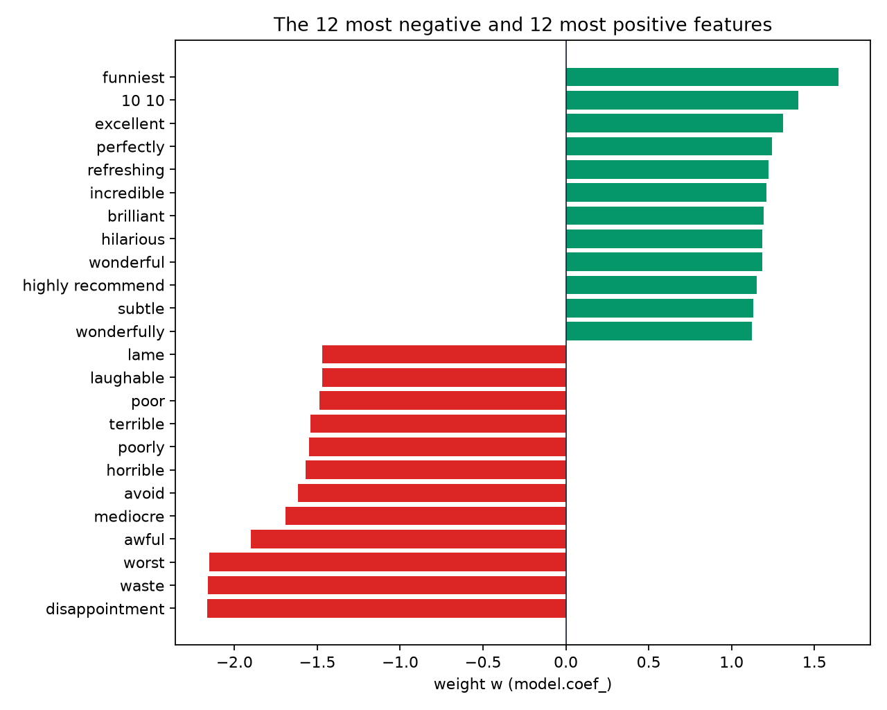
The most negative weights belong to disappointment (-2.1646), waste (-2.1606) and worst (-2.1519); the most positive to funniest (1.6471), the bigram 10 10 (1.4037, as in a rating of "10/10") and excellent (1.3094).
Worked example: long lines and poor customer service
The scenario's negative review is Long lines and poor customer service. Score it with the trained model. Weights are rounded to 4 decimals.
Step 1: which features does the model see?
Predict first: which word is a stop word, and do any bigrams survive?
and is a stop word. The five words that remain are all in the vocabulary, while the four bigrams (long lines, lines poor, poor customer, customer service) are not. Each word appears once, so every x is 1:
| Feature | x | Weight w | w·x |
|---|---|---|---|
| customer | 1 | -0.1980 | -0.1980 |
| lines | 1 | -0.1184 | -0.1184 |
| long | 1 | -0.0284 | -0.0284 |
| poor | 1 | -1.4874 | -1.4874 |
| service | 1 | -0.4832 | -0.4832 |
Step 2: compute z
Σ w·x = -0.1980 - 0.1184 - 0.0284 - 1.4874 - 0.4832 = -2.3154
z = -0.0488 + (-2.3154) = -2.3642
Every weight is negative, and poor alone gives almost two thirds of the sum.
Step 3: the sigmoid and the decision
e^(2.3642) = 10.6355
p = 1 / (1 + 10.6355) = 0.0859
p = 0.0859 is below 0.5, so the prediction is negative. The notebook's predict_proba gives 0.08594: close to 0, as the scenario says.
Worked example: best meal I've ever had
The scenario's positive review is Best meal I've ever had and awesome service, too! The plan says it "might score 0.9 or higher". Predict: does this model agree?
Step 1: the features
I is too short, and ever, had, and and too are stop words. Five words remain, and no bigram is in the vocabulary:
| Feature | x | Weight w | w·x |
|---|---|---|---|
| awesome | 1 | 0.7310 | 0.7310 |
| best | 1 | 0.7090 | 0.7090 |
| meal | 1 | 0.0062 | 0.0062 |
| service | 1 | -0.4832 | -0.4832 |
| ve | 1 | -0.0820 | -0.0820 |
Step 2: z and p
Σ w·x = 0.7310 + 0.7090 + 0.0062 - 0.4832 - 0.0820 = 0.8810
z = -0.0488 + 0.8810 = 0.8322
e^(-0.8322) = 0.4351
p = 1 / (1 + 0.4351) = 0.6968
The prediction is positive, but the score is 0.6968, not 0.9. predict_proba gives the same 0.69682.
Why not 0.9?
- The model learned from movie reviews. In movie reviews
serviceis a negative word (-0.4832), and it pulls this restaurant review down. - Short texts have few features, so the sum
Σ w·xstays small andpstays near the middle. - The 0.9 in the plan describes what a sentiment score means; the actual number always depends on the data the model was trained on.
Open the sentiment meter full screen. Type any review, or pick one of the examples, and press Play to add the words one at a time: stop words are crossed out, words outside the vocabulary are dashed, and each known word colours the text by its weight while the needle moves.
Part 4: The notebook in Colab
Open the notebook
Open Sentiment Analysis in Colab
The notebook needs three small changes to run in Colab today:
- It reads
Data/reviews.csv, a folder that does not exist next to the notebook in Colab. Read the file from the repository instead (about 65 MB). - It calls
plot_confusion_matrix, which was removed from scikit-learn. UseConfusionMatrixDisplay.from_estimator. - It saves the model into
Data/. Save it in the current folder instead.
Load the data and remove duplicates
import pandas as pd

url = ("https://raw.githubusercontent.com/"
       "jeffprosise/Machine-Learning/master/Data/reviews.csv")
df = pd.read_csv(url, encoding="ISO-8859-1")
df.info()
df.groupby('Sentiment').describe()df.info()reports 50,000 rows and two columns,TextandSentiment, with no missing values.describe()shows 25,000 reviews of each class, but only 24,697 unique negative texts and 24,884 unique positive ones.
df = df.drop_duplicates()
df.groupby('Sentiment').describe()
After drop_duplicates() there are 49,581 reviews: 24,697 negative and 24,884 positive. That removed 303 negative and 116 positive duplicates, 419 rows in total. The two classes are still almost balanced.
Vectorize and split
from sklearn.feature_extraction.text import CountVectorizer

vectorizer = CountVectorizer(ngram_range=(1, 2), stop_words='english', min_df=20)
x = vectorizer.fit_transform(df['Text'])
y = df['Sentiment']

from sklearn.model_selection import train_test_split

x_train, x_test, y_train, y_test = train_test_split(x, y, test_size=0.5, random_state=0)x.shapeis(49581, 33752): 17,528 unigrams and 16,224 bigrams passedmin_df=20.- The notebook splits 50/50 because the dataset is large: 24,790 reviews to train and 24,791 to test (12,422 positive and 12,369 negative).
Train the model
from sklearn.linear_model import LogisticRegression

model = LogisticRegression(max_iter=1000, random_state=0)
model.fit(x_train, y_train)
fit learns one weight per vocabulary entry, 33,752 weights, plus the bias b. max_iter=1000 gives the solver enough iterations to converge on this many features; our run needed 78.
The confusion matrix
from sklearn.metrics import ConfusionMatrixDisplay

ConfusionMatrixDisplay.from_estimator(model, x_test, y_test,
    display_labels=['Negative', 'Positive'], cmap='Blues', xticks_rotation='vertical')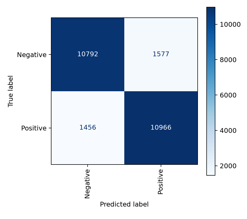
| Predicted negative | Predicted positive | |
|---|---|---|
| Actual negative | 10,792 | 1,577 |
| Actual positive | 1,456 | 10,966 |
The model correctly identified 10,792 negative reviews and misclassified 1,577 of them; it correctly identified 10,966 positive reviews and got 1,456 wrong.
The saved notebook shows 10,795 and 1,574 in the first row, and a few of its printed numbers differ in the third or fourth decimal. That notebook was run with an older version of scikit-learn; every number on this page comes from our own run with scikit-learn 1.9.1, and your Colab numbers can also differ by a few reviews.
Worked example: score the model
Compute the accuracy A, and the precision P and recall R of the positive class, from the matrix. Try it before reading on.
A = (10792 + 10966) / 24791 = 21758 / 24791 = 0.8777
P = 10966 / (10966 + 1577) = 10966 / 12543 = 0.8743
R = 10966 / (10966 + 1456) = 10966 / 12422 = 0.8828
model.score(x_test, y_test) prints 0.8776572143116453, the same accuracy. About 88 of every 100 test reviews are classified correctly.
ROC AUC
The notebook then asks for a better measure than accuracy:
from sklearn.metrics import roc_auc_score

probabilities = model.predict_proba(x_test)
roc_auc_score(y_test, probabilities[:, 1])
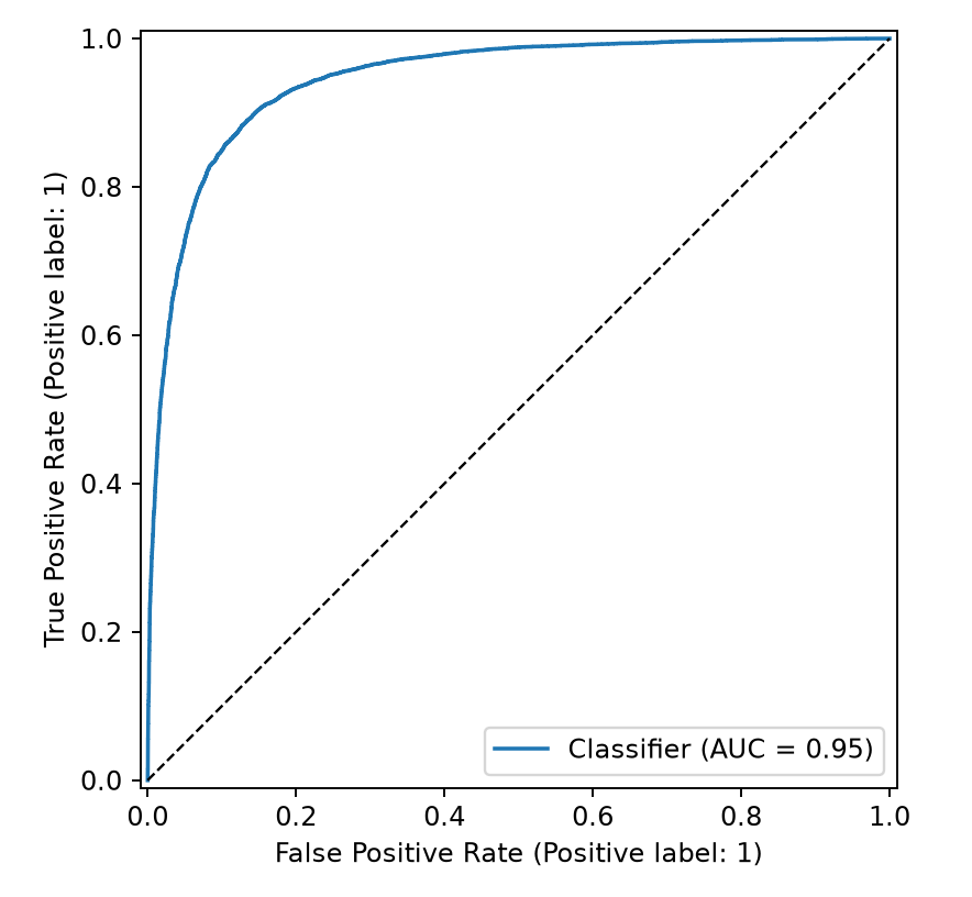
The output is 0.9451676789628598. Accuracy judges the predictions at one threshold, 0.5. The area under the ROC curve judges the scores at every threshold: 1.0 would be perfect and 0.5 is guessing. It also has a direct meaning: take one random positive review and one random negative review; the model gives the positive one the higher score in about 94.5 percent of such pairs.
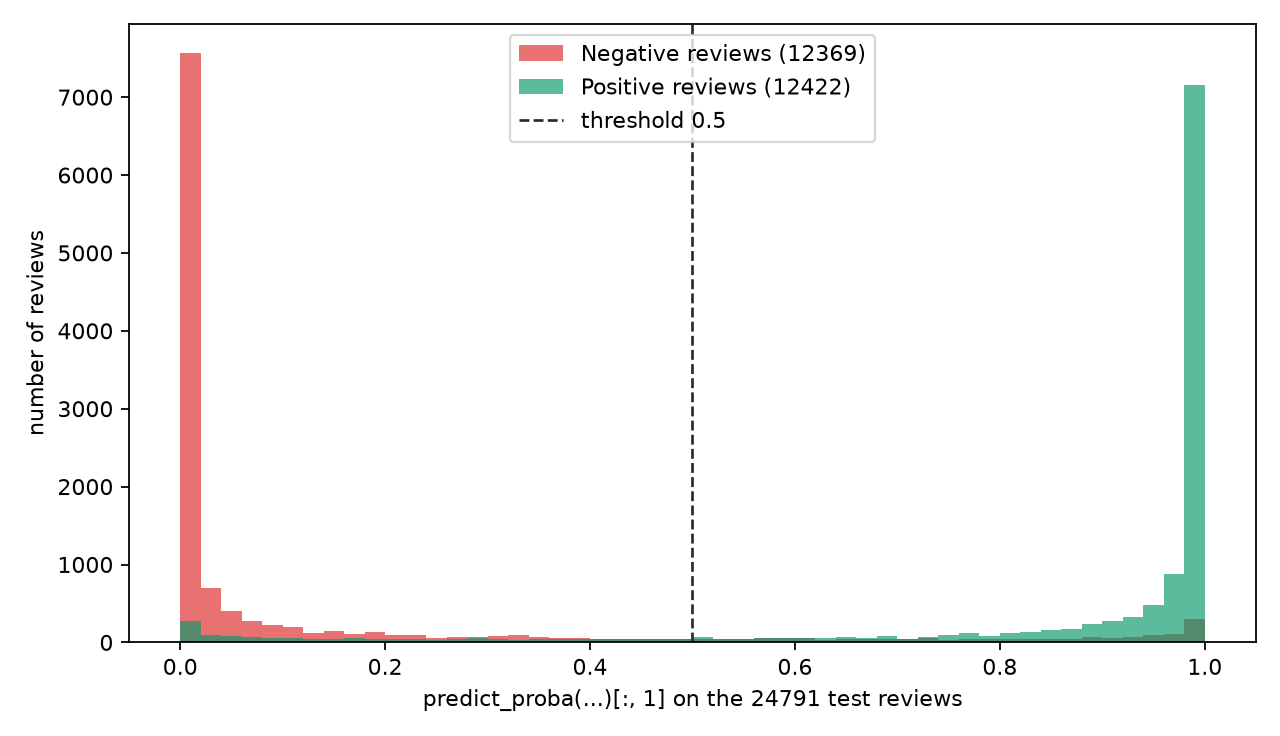
The scores are well separated. Most test reviews score close to 0 or close to 1, and only 3.9 percent fall between 0.4 and 0.6:
Moving the threshold trades precision against recall, as in week 4:
| Threshold t | TN, FP, FN, TP | Accuracy | Precision (positive) | Recall (positive) |
|---|---|---|---|---|
| 0.3 | 10232, 2137, 1028, 11394 | 0.8723 | 0.8421 | 0.9172 |
| 0.5 | 10792, 1577, 1456, 10966 | 0.8777 | 0.8743 | 0.8828 |
| 0.7 | 11251, 1118, 2054, 10368 | 0.8721 | 0.9027 | 0.8346 |
Open the threshold and ROC widget full screen. Drag the threshold across the histogram of the test scores, watch the confusion matrix and the point on the ROC curve move together, and press Sweep to trace the whole curve.
Score new reviews
reviews = ['Long lines and poor customer service',
           "Best meal I've ever had and awesome service, too!"]
model.predict_proba(vectorizer.transform(reviews))[:, 1]
[0.08594148 0.69681757]These are the two worked examples. Always call transform, never fit_transform, on new text: the model only knows the vocabulary it was trained with. The notebook scores two more reviews:
| Review | Score p |
|---|---|
| The long lines and poor customer service really turned me off. | 0.0915 |
| One of the more delightful experiences I have had! | 0.7025 |
In the second one, one, of, the, more, I, have and had are all removed; only delightful (0.8111) and experiences (0.0968) are left to decide.
Save the model
import pickle

pickle.dump(model, open('sentiment.pkl', 'wb'))
pickle.dump(vectorizer.vocabulary_, open('vocabulary.pkl', 'wb'))
The notebook saves the trained model and the vocabulary, so an application can load them and score text without training again. Saving the vocabulary matters: without it, new text cannot be turned into the same 33,752 columns.
Part 5: Where a bag of words goes wrong
The model is 88 percent accurate on movie reviews, yet it is easy to fool. Try these in the sentiment meter.
Negation is thrown away
not is in the English stop list, so it is removed before the model sees the text:
| Review | Features | Score p |
|---|---|---|
| The food was good | food, good | 0.5885 |
| The food was not good | food, good | 0.5885 |
Both reviews become the same count vector, so they get the same score.
Word order is thrown away
| Review | Score p |
|---|---|
| Great food but terrible service | 0.2591 |
| Terrible food but great service | 0.2591 |
A bag of words only counts, so the two reviews are identical to the model. None of their bigrams (great food, terrible service, ...) is in the vocabulary, so even the pairs cannot help.
The training data decides the weights
The model learned from movie reviews. service (-0.4832) and staff (-0.4587) carry negative weights, while rude is only -0.0364. A restaurant company would get better scores by training on labelled restaurant reviews, with exactly the same code.
Common mistakes
- Reading
Data/reviews.csvin Colab from a folder that does not exist there. - Calling
plot_confusion_matrix: it was removed; useConfusionMatrixDisplay.from_estimator. - Calling
fit_transformon new reviews. New text needsvectorizer.transform([...])with the vocabulary learned from the training text. - Passing a plain string to
transform. It needs a list of texts:transform([review]). - Reading
predict_proba(...)[0][0]as the sentiment score. Column1is the probability of positive:[0][1], or[:, 1]for many reviews. - Expecting
notto flip a score whilestop_words='english'removes it.
Project milestone: presentations and discussions
This week's milestone is Project Teams Presentations and Discussions: each team presents its project and discusses it. Next week is the final submission, which the plan lists as:
- The project code on a GitHub repository.
- A project video, 5 minutes long.
- The project proposal.
- The project presentation.
- The project logo.
- Additionally, a user interface for the project (mobile, web or desktop).
If your project works with text, today's pipeline applies directly: vectorize with CountVectorizer, train a classifier, score with predict_proba, and save both the model and the vocabulary.
Key takeaways
- Sentiment analysis is binary classification: the score is
p, the probability of the positive class. CountVectorizerturns text into counts: lower case, tokens, stop words removed, unigrams and bigrams, only the vocabulary kept.- The score is
σ(b + Σ w·x): each known word pushes by its weight, and unknown words and stop words do nothing. - The notebook's model reaches an accuracy of 0.8777 and a ROC AUC of 0.9452 on 24,791 test reviews.
- A bag of words ignores order and, with stop words removed, negation; the weights reflect the data it was trained on.
Practice
About 30 minutes. Try each task before you read its answer at the end of the page.
Practice 1: vectorize by hand (about 5 minutes)
Review: The waiter was rude and the food was cold.
- List the tokens after lower case.
- Remove the stop words (
the,wasandandare stop words). - List every unigram and bigram that
ngram_range=(1, 2)would build.
Practice 2: score two reviews by hand (about 10 minutes)
Use b = -0.0488 and these weights from the trained model. For each review, compute Σ w·x, z, p and the prediction at threshold 0.5.
| Feature | Weight w |
|---|---|
| waiter | -0.0937 |
| rude | -0.0364 |
| food | 0.2302 |
| cold | -0.2052 |
| excellent | 1.3094 |
| friendly | 0.1913 |
| staff | -0.4587 |
| highly | 0.6243 |
| recommend | 0.3000 |
| highly recommend | 1.1524 |
- The waiter was rude and the food was cold. Only the four single words are in the vocabulary.
- Excellent food, friendly staff, highly recommend! All six words are in the vocabulary, and so is one bigram.
Practice 3: choose a threshold (about 5 minutes)
A restaurant chain wants to find as many negative reviews as possible so a manager can reply to each one. Here are the model's results on the 24,791 test reviews:
| Threshold t | TN | FP | FN | TP |
|---|---|---|---|---|
| 0.3 | 10232 | 2137 | 1028 | 11394 |
| 0.7 | 11251 | 1118 | 2054 | 10368 |
- For each threshold, compute the recall of the negative class,
TN / (TN + FP). - Which threshold finds more negative reviews? What does the chain pay for it?
Practice 4: in Colab (about 10 minutes)
- Run the notebook with the three changes, and score the two scenario reviews in one call to
predict_proba. - Score
The food was goodandThe food was not good. - Build a second vectorizer that keeps the stop words:
CountVectorizer(ngram_range=(1, 2), min_df=20). Refit, split with the samerandom_state=0, retrain, and print the number of features, the accuracy and the ROC AUC. - Score the two food reviews again with the new model. What changed, and why?
Answers
Answer 1
- Tokens:
the, waiter, was, rude, and, the, food, was, cold. The full stop disappears. - After removing the stop words:
waiter, rude, food, cold. - Unigrams and bigrams, 7 in total:
waiter, rude, food, cold, waiter rude, rude food, food cold. The bigramrude foodexists only because the stop words between the two words were removed first.
Answer 2
Review 1: The waiter was rude and the food was cold.
Σ w·x = -0.0937 - 0.0364 + 0.2302 - 0.2052 = -0.1051
z = -0.0488 + (-0.1051) = -0.1539
e^(0.1539) = 1.1664
p = 1 / (1 + 1.1664) = 0.4616
p is below 0.5, so the prediction is negative, but only just. rude is barely negative in movie reviews, and food is positive. predict_proba gives 0.4616 as well.
Review 2: Excellent food, friendly staff, highly recommend!
Σ w·x = 1.3094 + 0.2302 + 0.1913 - 0.4587 + 0.6243 + 0.3000 + 1.1524 = 3.3489
z = -0.0488 + 3.3489 = 3.3001
e^(-3.3001) = 0.0369
p = 1 / (1 + 0.0369) = 0.9644
The prediction is positive with p = 0.9644. The bigram highly recommend (1.1524) counts on top of highly and recommend. predict_proba gives 0.9644.
Answer 3
- t = 0.3:
10232 / (10232 + 2137) = 10232 / 12369 = 0.8272. - t = 0.7:
11251 / (11251 + 1118) = 11251 / 12369 = 0.9096.
The higher threshold, 0.7, finds more negative reviews: a review is called positive only when p ≥ 0.7, so more reviews are called negative. The price is that more positive reviews are called negative too: FN grows from 1028 to 2054, so the manager reads more reviews that did not need a reply.
Answer 4
- The two scenario reviews score
[0.08594148 0.69681757]. - Both food reviews score 0.5885:
notis removed as a stop word, so both reviews becomefood, good. - With the stop words kept, our run gives 74,938 features, an accuracy of 0.8967 and a ROC AUC of 0.9574, both higher than 0.8777 and 0.9452.
The food was goodnow scores 0.7082 andThe food was not goodscores 0.2912. The new vocabulary containsnot(-0.1181),was not(-0.2283) and the bigramnot good(-0.7838), so negation can finally push the score down. The price is a vocabulary more than twice as large.