

Linear Regression
This section introduces the first real prediction model of the course: linear regression. It predicts a number, here the price of a house, from one or more input numbers by fitting a straight line (or its many-feature version) to the data. You will first fit a line by hand to five real houses with the least-squares method, then explore, clean and model a dataset of 5000 houses with the week 3 notebook, and judge the model with its error measures.
Objectives
By the end of the section you should be able to:
- Explain what linear regression predicts, and the difference between simple and multiple linear regression.
- Define a residual and the least-squares line, and compute the slope and the intercept by hand.
- Compute MAE, MSE, RMSE and R² for a fitted line.
- Explore a dataset with
info,describe, a histogram and a correlation heatmap, and prepare it for a model. - Fit
LinearRegressionin scikit-learn, read its intercept and coefficients, and predict a new house by hand from them. - Evaluate the model on test data with plots of the residuals and the error measures, and apply the same steps to your team project.
Where this sits in the course
Week 3 of the plan has three parts:
- The notebook.
Linear_Regression_Practicefrom the course repository, which models the prices of 5000 houses in the USA. - A real-world scenario. Predict House Pricing.
- A project milestone. Project Data Exploration and Data Cleaning: this week your team explores and cleans its own dataset.
In week 2, sns.regplot drew the straight line that fits a scatter plot best. This week you learn how that line is found and how to use it to predict.
| Part | What we do | Time |
|---|---|---|
| 1 | The idea, least squares, and a worked example by hand | 35 min |
| 2 | Notebook: explore and prepare the housing data | 20 min |
| 3 | Notebook: fit the model and read its coefficients | 20 min |
| 4 | Evaluate the model on the test set, your project | 15 min |
| 5 | Practice with answers, then takeaways | 30 min |
Part 1: The idea of linear regression
What linear regression is
The notebook opens with this definition: linear regression is a linear approach for modeling the relationship between a scalar dependent variable y and one or more explanatory variables (or independent variables) denoted X.
- With one explanatory variable it is called simple linear regression.
- With more than one it is called multiple linear regression.
- Linear regression models are often fitted using the least squares approach.
In the house-pricing scenario, y is the price of a house and X holds numbers that describe its area, such as the average income of the people who live there.
The model is a straight line
With one feature x, the model is a line:
ŷ = b0 + b1 · xxis the input, for example the average income of the area.ŷ(read "y hat") is the predicted value, for example the predicted price.b1is the slope: how muchŷchanges whenxgrows by 1.b0is the intercept: the value ofŷwhenx = 0. It places the line up or down.
With five features x1 to x5, the same idea becomes ŷ = b0 + b1·x1 + b2·x2 + b3·x3 + b4·x4 + b5·x5, one coefficient per feature. That is the model of the notebook.
Residuals
For a data point with true value y and prediction ŷ, the residual is the error of the prediction:
e = y - ŷA point above the line has a positive residual, a point below it a negative one. On a plot, the residual is the vertical distance from the point to the line.
Least squares
Many lines pass near the points. The least-squares line is the one whose squared residuals have the smallest possible sum:
SSE = e1² + e2² + ... + en² = Σ (yi - ŷi)²SSE is the sum of squared errors and n is the number of points. Squaring makes every error count as positive and punishes big errors more than small ones. For one feature, the slope and the intercept that make SSE smallest are:
b1 = Σ (xi - x̄)(yi - ȳ) / Σ (xi - x̄)²

b0 = ȳ - b1 · x̄
x̄ and ȳ are the means of x and y. The second formula means the least-squares line always passes through the point (x̄, ȳ).
Worked example: five houses, by hand
We take five real houses from the notebook's dataset, USA_Housing.csv. To keep the arithmetic small we measure the income in units of 100,000, and round both to whole units.
| House | Row in the dataset | Avg. Area Income | Price | x | y |
|---|---|---|---|---|---|
| H1 | 4034 | $50,016.43 | $497,368.04 | 5 | 5 |
| H2 | 375 | $59,768.81 | $897,291.12 | 6 | 9 |
| H3 | 1920 | $69,528.56 | $995,137.20 | 7 | 10 |
| H4 | 427 | $79,627.63 | $1,196,064.33 | 8 | 12 |
| H5 | 4841 | $89,548.15 | $1,403,802.50 | 9 | 14 |
Question. Find the least-squares line ŷ = b0 + b1·x, measure its error, and predict the price of an area with an average income of $75,000.
Step 1: the means
x̄ = (5 + 6 + 7 + 8 + 9) / 5 = 35 / 5 = 7

ȳ = (5 + 9 + 10 + 12 + 14) / 5 = 50 / 5 = 10
Step 2: deviations from the means
| House | x - x̄ | y - ȳ | (x - x̄)(y - ȳ) | (x - x̄)² |
|---|---|---|---|---|
| H1 | -2 | -5 | 10 | 4 |
| H2 | -1 | -1 | 1 | 1 |
| H3 | 0 | 0 | 0 | 0 |
| H4 | 1 | 2 | 2 | 1 |
| H5 | 2 | 4 | 8 | 4 |
| Sum | 21 | 10 |
Step 3: slope and intercept
b1 = 21 / 10 = 2.1

b0 = ȳ - b1 · x̄ = 10 - 2.1 × 7 = 10 - 14.7 = -4.7
The least-squares line is ŷ = -4.7 + 2.1x. The slope means that each extra 210,000**, to the predicted price. The intercept, -4.7, is the price the line gives at an income of zero; no area has that income, so it only positions the line.
scikit-learn agrees: LinearRegression().fit(xh, yh) on these five points gives intercept_ = -4.7 and coef_ = [2.1]. On all 3500 training houses of the notebook, a model with income as its only feature gets a coefficient of 20.9961 dollars of price per dollar of income, that is 10,000: almost the same slope as our five houses.
Step 4: predictions and residuals
| House | x | y | ŷ = -4.7 + 2.1x | e = y - ŷ | e² |
|---|---|---|---|---|---|
| H1 | 5 | 5 | 5.8 | -0.8 | 0.64 |
| H2 | 6 | 9 | 7.9 | 1.1 | 1.21 |
| H3 | 7 | 10 | 10.0 | 0.0 | 0.00 |
| H4 | 8 | 12 | 12.1 | -0.1 | 0.01 |
| H5 | 9 | 14 | 14.2 | -0.2 | 0.04 |
The residuals add up to -0.8 + 1.1 + 0 - 0.1 - 0.2 = 0. That is always true for a least-squares line with an intercept, and it is a quick check of your arithmetic.
Step 5: the sum of squared errors
SSE = 0.64 + 1.21 + 0 + 0.01 + 0.04 = 1.90Compare it with two lines you might guess by eye:
| Line | Residuals | SSE |
|---|---|---|
| ŷ = -3 + 2x | -2, 0, -1, -1, -1 | 7.0 |
| ŷ = -4 + 2x | -1, 1, 0, 0, 0 | 2.0 |
| ŷ = -4.7 + 2.1x (least squares) | -0.8, 1.1, 0, -0.1, -0.2 | 1.9 |
The second guess looks perfect on three houses, yet its SSE is 2.0. No line can go below 1.9 for these five houses: that is what "least squares" means.
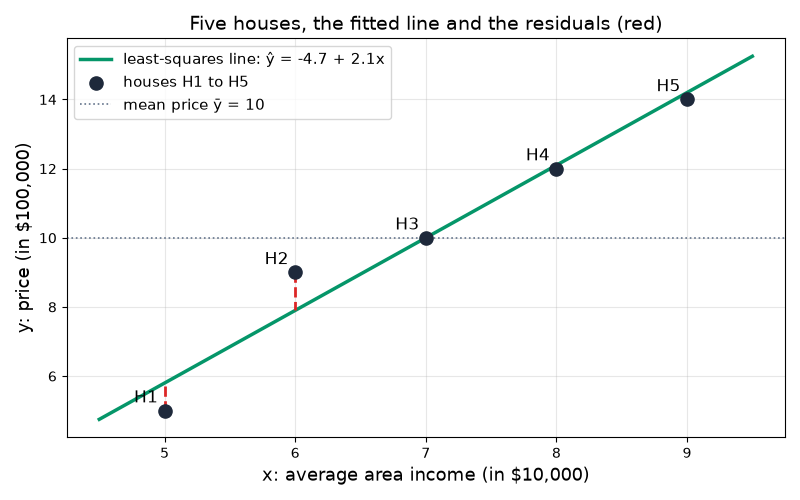
Step 6: predict a new area
An average income of $75,000 is x = 7.5:
ŷ = -4.7 + 2.1 × 7.5 = -4.7 + 15.75 = 11.05The predicted price is 11.05 units, that is about $1,105,000. model.predict([[7.5]]) returns the same 11.05.
To see least squares move, open the least-squares playground full screen. Drag the houses or the line, switch on the squares, press Play to add the squared residuals one house at a time, and press Fit to move the line to the least-squares line.
Measuring the error of a line
The notebook evaluates its model with four numbers. With n points and residuals ei:
MAE  = (|e1| + |e2| + ... + |en|) / n
MSE  = (e1² + e2² + ... + en²) / n = SSE / n
RMSE = √MSE
R² = 1 - SSE / SST, where SST = Σ (yi - ȳ)²- MAE, mean absolute error: the average size of an error, in the units of
y. - MSE, mean squared error: the average squared error. Its unit is the square of the unit of
y, so it is hard to read on its own. - RMSE, root mean squared error: the square root of MSE, back in the units of
y. Big errors weigh more in it than in MAE. - R², the coefficient of determination:
SSTis the SSE of the flat lineŷ = ȳ, the best guess you can make without any feature. R² is the share of that error the model removes. 1 is a perfect fit, 0 is no better than the mean.
Worked example: the error of the five-house line
Question. Compute MAE, MSE, RMSE and R² for ŷ = -4.7 + 2.1x.
MAE  = (0.8 + 1.1 + 0 + 0.1 + 0.2) / 5 = 2.2 / 5 = 0.44
MSE  = 1.90 / 5 = 0.38
RMSE = √0.38 = 0.6164
In dollars, the RMSE is 0.6164 × $100,000, about $61,640.
For R², first the squared deviations of y from ȳ = 10: 25, 1, 0, 4, 16.
SST = 25 + 1 + 0 + 4 + 16 = 46
R²  = 1 - 1.90 / 46 = 1 - 0.0413 = 0.9587
The line removes about 96% of the squared error of the flat line at the mean price. scikit-learn's metrics functions give the same four values: 0.44, 0.38, 0.6164 and 0.9587.
Open the R² widget full screen to watch the flat mean line tilt into the least-squares line while SSE shrinks, on these five houses and on 60 real houses with each of the five features.
Part 2: Notebook, exploring the housing data
Open the notebook
Open Linear_Regression_Practice in Colab
The notebook reads the data with pd.read_csv("./Datasets/USA_Housing.csv"). In Colab there is no Datasets folder next to the notebook: in the repository the file lives in the Datasets folder at the top level. Read it from the repository instead:
import numpy as np
import pandas as pd
import matplotlib.pyplot as plt
import seaborn as sns

url = ("https://raw.githubusercontent.com/"
       "tirthajyoti/Machine-Learning-with-Python/"
       "master/Datasets/USA_Housing.csv")
df = pd.read_csv(url)
df.head()
Check the basic info
df.info(verbose=True) reports 5000 rows and 7 columns:
| Column | Type | Meaning |
|---|---|---|
| Avg. Area Income | float64 | average income of the residents of the area, in dollars |
| Avg. Area House Age | float64 | average age of the houses in the area, in years |
| Avg. Area Number of Rooms | float64 | average number of rooms per house |
| Avg. Area Number of Bedrooms | float64 | average number of bedrooms per house |
| Area Population | float64 | number of people living in the area |
| Price | float64 | the price of the house, the value we predict |
| Address | text | the address, for example 208 Michael Ferry Apt. 674 |
Every column shows 5000 non-null, so there are no missing values; df.isnull().sum() confirms a 0 for every column. Address is text, and a linear model can only multiply numbers, so it will be left out of X.
The statistical summary
df.describe(percentiles=[0.1,0.25,0.5,0.75,0.9]) summarizes every numeric column. Four rows for the two columns we use most:
| Statistic | Avg. Area Income | Price |
|---|---|---|
| mean | 68,583.11 | 1,232,073 |
| std | 10,657.99 | 353,118 |
| min | 17,796.63 | 15,939 |
| max | 107,701.75 | 2,469,066 |
pandas prints the price in scientific notation, for example 1.232073e+06, which means 1.232073 × 10⁶, that is 1,232,073.
The distribution of the price
df['Price'].plot.hist(bins=25, figsize=(8,4))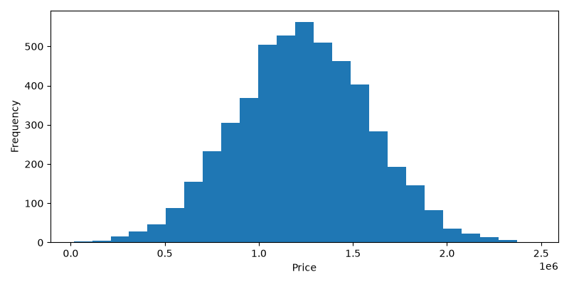
The prices form one hill around the mean of about 0.5 million and 74 more than $2 million. The 1e6 under the axis means that the tick labels are in millions. The notebook also draws the same distribution as a smooth curve with df['Price'].plot.density().
Correlations
The notebook calls df.corr(). In current pandas this line stops with ValueError: could not convert string to float, because Address is text. Ask for the numeric columns only:
df.corr(numeric_only=True)

plt.figure(figsize=(10,7))
sns.heatmap(df.corr(numeric_only=True), annot=True, linewidths=2)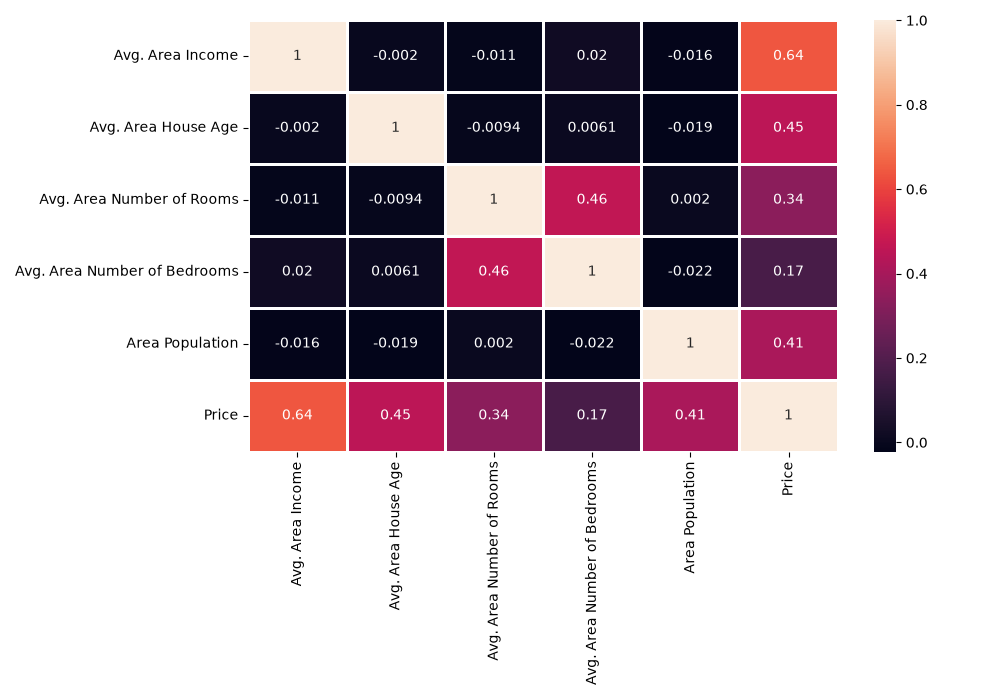
Read the Price row. Every feature has a positive correlation with the price:
| Feature | Correlation with Price |
|---|---|
| Avg. Area Income | 0.640 |
| Avg. Area House Age | 0.453 |
| Area Population | 0.409 |
| Avg. Area Number of Rooms | 0.336 |
| Avg. Area Number of Bedrooms | 0.171 |
Income moves most with the price and bedrooms least. The features hardly correlate with each other (values near 0), except rooms and bedrooms at 0.46, which makes sense: houses with more rooms tend to have more bedrooms. The notebook also draws sns.pairplot(df), a grid of every pair of columns, and one scatter plot of each feature against the price:
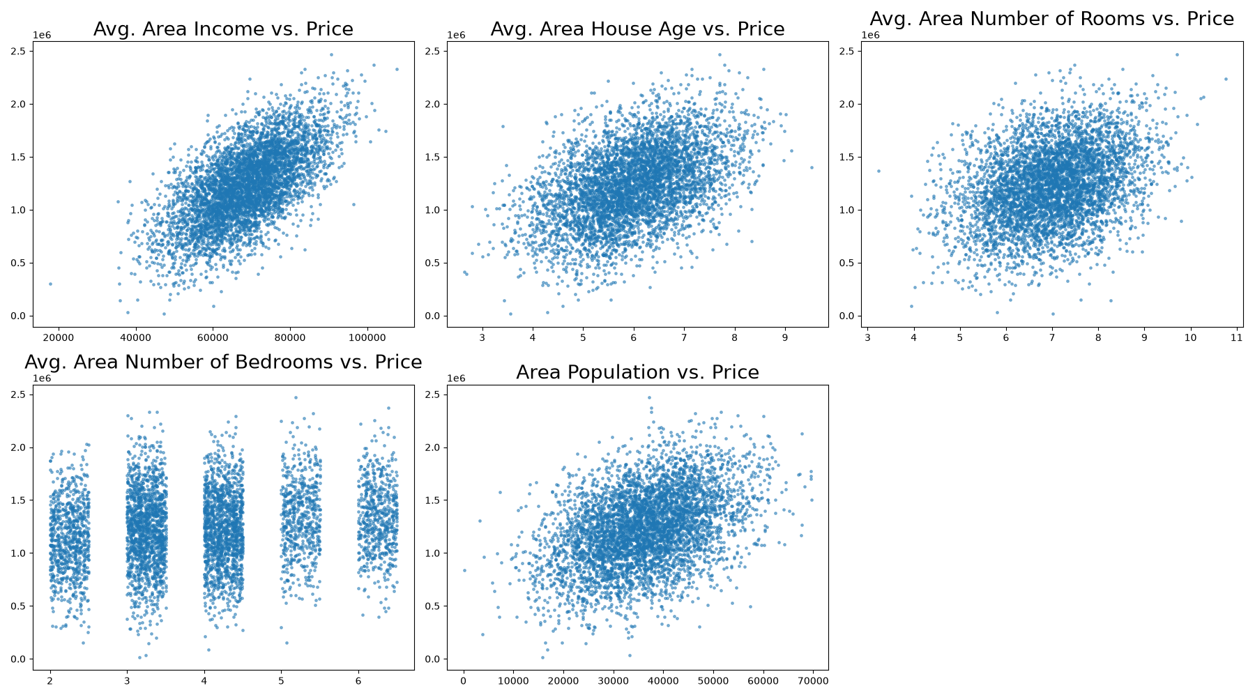
The income panel shows the clearest upward trend. The bedrooms panel shows vertical bands just above each whole number, with almost the same prices in every band.
Part 3: Notebook, fitting the model
Features and target
l_column = list(df.columns)
len_feature = len(l_column)
X = df[l_column[0:len_feature-2]]
y = df[l_column[len_feature-2]]
print("Feature set size:", X.shape)
print("Variable set size:", y.shape)
The list of columns has 7 names, so len_feature - 2 = 5. X takes columns 0 to 4, the five numeric features, and y takes column 5, Price. Address, the last column, is left out. The output:
Feature set size: (5000, 5)
Variable set size: (5000,)
Train and test split
The notebook imports train_test_split from sklearn.cross_validation. That module was removed from scikit-learn long ago, so the import fails; the function now lives in sklearn.model_selection:
from sklearn.model_selection import train_test_split
X_train, X_test, y_train, y_test = train_test_split(
    X, y, test_size=0.3, random_state=123)
test_size=0.3 keeps 30% of the rows for testing: 0.3 × 5000 = 1500 test houses and 3500 training houses. The shapes print as (3500, 5) and (1500, 5).
Fit and read the coefficients
from sklearn.linear_model import LinearRegression
from sklearn import metrics

lm = LinearRegression()
lm.fit(X_train, y_train)
print("The intercept term of the linear model:", lm.intercept_)

cdf = pd.DataFrame(data=lm.coef_, index=X_train.columns, columns=["Coefficients"])
cdf
The intercept is -2631028.9017454907, and the coefficients are:
| Feature | Coefficient |
|---|---|
| Avg. Area Income | 21.597602 |
| Avg. Area House Age | 165201.104954 |
| Avg. Area Number of Rooms | 119061.463868 |
| Avg. Area Number of Bedrooms | 3212.585606 |
| Area Population | 15.228121 |
So the fitted model is:
ŷ = -2631028.90 + 21.597602·x1 + 165201.104954·x2 + 119061.463868·x3 + 3212.585606·x4 + 15.228121·x5where x1 to x5 are income, house age, rooms, bedrooms and population, in the order of the table.
Each coefficient is the change in the predicted price when that one feature grows by 1 and the other four stay the same:
- One more year of average house age adds $165,201.10.
- One more room adds $119,061.46.
- One more dollar of area income adds **10,000 more income adds $215,976.
A coefficient depends on the unit of its feature. Income is measured in dollars, so its coefficient looks small, yet income is the feature that moves the price most. Do not rank features by the size of their coefficients.
Worked example: predict one test house by hand
Question. The first test house is row 2648 of the dataset. Predict its price from the coefficients, then compare with its real price, $800,146.23.
| Feature | Value x | Coefficient b | b × x |
|---|---|---|---|
| Avg. Area Income | 63824.394539 | 21.597602 | 1,378,453.87 |
| Avg. Area House Age | 4.991750 | 165201.104954 | 824,642.62 |
| Avg. Area Number of Rooms | 5.003836 | 119061.463868 | 595,764.04 |
| Avg. Area Number of Bedrooms | 4.00 | 3212.585606 | 12,850.34 |
| Area Population | 40086.458749 | 15.228121 | 610,441.44 |
Σ b × x = 1,378,453.87 + 824,642.62 + 595,764.04 + 12,850.34 + 610,441.44 = 3,422,152.31
ŷ = -2,631,028.90 + 3,422,152.31 = 791,123.41
e = 800,146.23 - 791,123.41 = 9,022.82
The model predicts about **800,146: the prediction is $9,023 too low. lm.predict(X_test)[0] prints 791123.50601188; the 10 cents of difference come from rounding the coefficients to six decimals. A fitted model is nothing more than this sum.
Which features matter most
The notebook computes a standard error for each coefficient and divides: t-statistic = coefficient / standard error. The larger the t-statistic, the more clearly the feature affects the price, whatever its unit. Its output, sorted:
| Feature | Coefficient | Standard error | t-statistic |
|---|---|---|---|
| Avg. Area Income | 21.597602 | 0.160361 | 134.681505 |
| Avg. Area House Age | 165201.104954 | 1722.412068 | 95.912649 |
| Area Population | 15.228121 | 0.169882 | 89.639472 |
| Avg. Area Number of Rooms | 119061.463868 | 1696.546476 | 70.178722 |
| Avg. Area Number of Bedrooms | 3212.585606 | 1376.451759 | 2.333962 |
Income matters most and bedrooms least, the same order as the correlations with the price. The fit on the training data gives R-squared value of this fit: 0.917.
One caution about this table: the notebook's standard error is a simplified formula that leaves out the correlation between the features. The exact standard errors of ordinary least squares (OLS) give a t-statistic of 62.37 for rooms (not 70.18) and 2.07 for bedrooms (not 2.33). The ranking stays the same.
Part 4: Evaluating the model on the test set
Predict the test houses
predictions = lm.predict(X_test)

plt.figure(figsize=(10,7))
plt.title("Actual vs. predicted house prices", fontsize=25)
plt.xlabel("Actual test set house prices", fontsize=18)
plt.ylabel("Predicted house prices", fontsize=18)
plt.scatter(x=y_test, y=predictions)
predictions is a NumPy array of 1500 prices, one per test house.
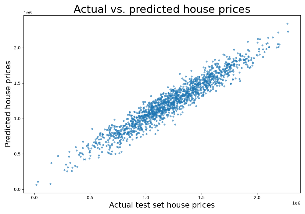
A perfect model would put every point on the 45 degree line where predicted equals actual. The points form a narrow band along that line: the model is close for cheap and for expensive houses alike.
Check the residuals
The notebook draws the residuals y_test - predictions twice. It uses sns.distplot, which current seaborn marks as deprecated; sns.histplot with kde=True draws the same picture:
plt.figure(figsize=(10,7))
plt.title("Histogram of residuals to check for normality", fontsize=25)
sns.histplot(y_test - predictions, kde=True)

plt.figure(figsize=(10,7))
plt.title("Residuals vs. predicted values plot (Homoscedasticity)", fontsize=20)
plt.scatter(x=predictions, y=y_test - predictions)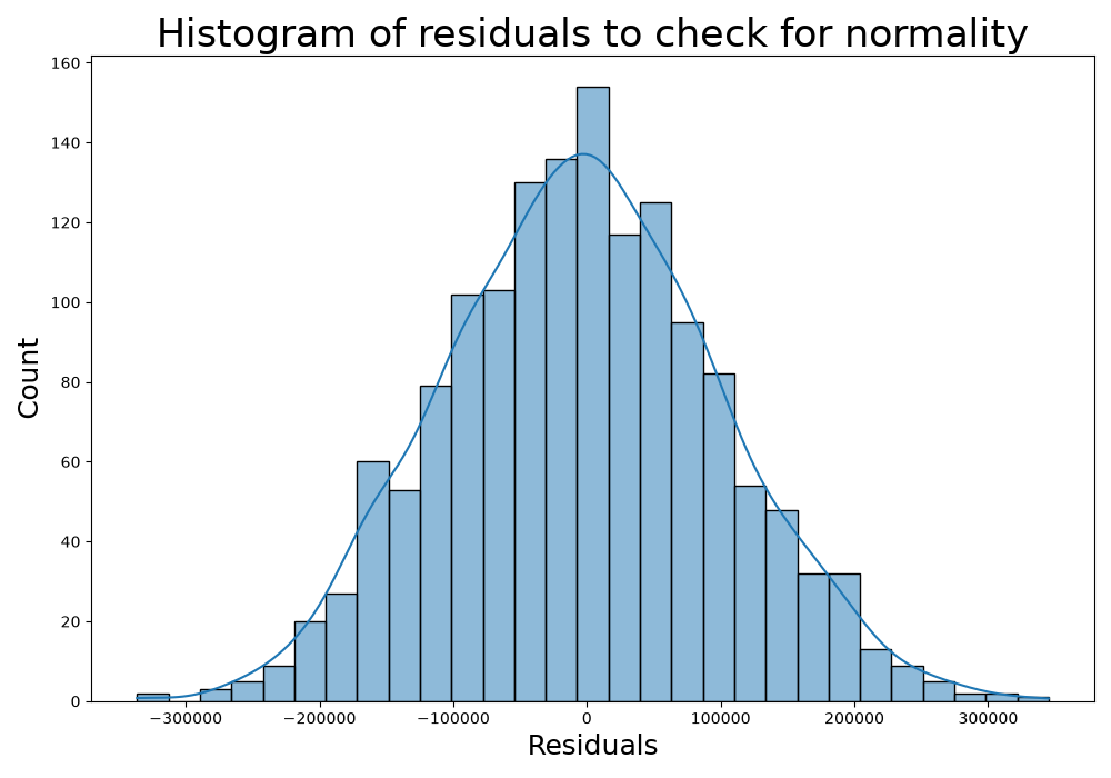
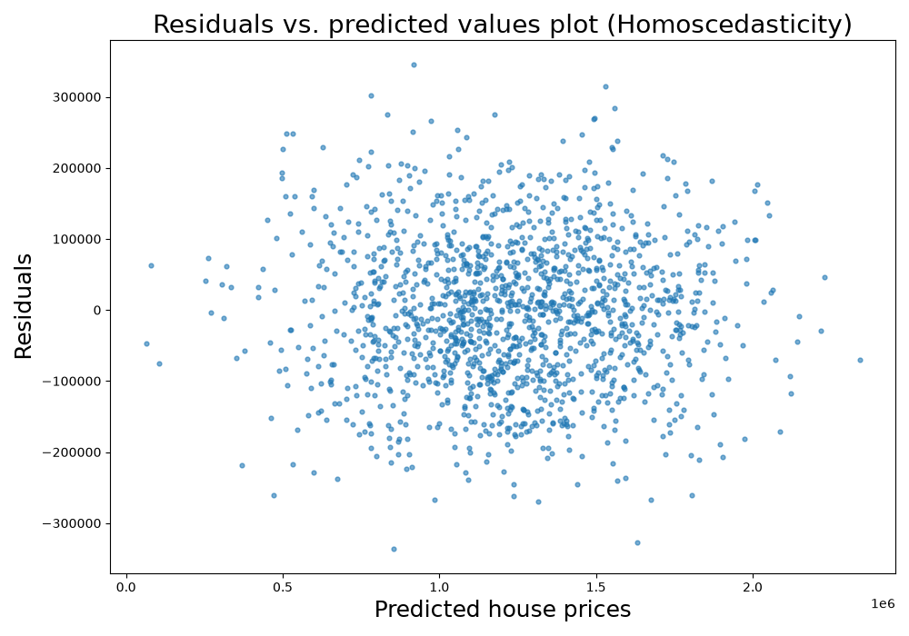
- The histogram is one symmetric hill centred near 0 (the mean residual is -336,000 to +$345,000.
- In the second plot the cloud has the same height for cheap and expensive predictions and shows no curve. The notebook calls this homoscedasticity: the size of the errors does not depend on the prediction.
The error measures
print("Mean absolute error (MAE):", metrics.mean_absolute_error(y_test, predictions))
print("Mean square error (MSE):", metrics.mean_squared_error(y_test, predictions))
print("Root mean square error (RMSE):", np.sqrt(metrics.mean_squared_error(y_test, predictions)))
print("R-squared value of predictions:", round(metrics.r2_score(y_test, predictions), 3))
Mean absolute error (MAE): 81739.77482718184
Mean square error (MSE): 10489638335.804983
Root mean square error (RMSE): 102418.93543581179
R-squared value of predictions: 0.919- MAE: on average a test prediction is off by about $81,740.
- MSE: about 10.5 billion squared dollars, a number with no everyday meaning.
- RMSE:
√10,489,638,335.80 = 102,418.94, so a typical error is about $102,419. It is larger than the MAE because the few large errors weigh more. - R²: 0.919 on the 1500 test houses, against 0.917 on the 3500 training houses. The model explains about 92% of the price spread on houses it never saw, and it does as well on new data as on its training data.
With a mean price of 102,419 is about 8% of the price.
Common mistakes
- Running the notebook's old calls as they are:
sklearn.cross_validation,df.corr()on a DataFrame with a text column, andsns.distplot. - Reading
./Datasets/USA_Housing.csvin Colab, where that folder does not exist. - Leaving the
Addresstext column inX. - Ranking features by the size of their coefficients when the features have different units.
- Reporting only the training R²; judge the model on the test set.
- Reading R² as an accuracy. It is the share of the squared error removed compared with predicting the mean.
- Trusting a prediction far outside the range of the training data, such as the intercept at an income of zero.
Project milestone: data exploration and data cleaning
This week's milestone is to explore and clean your team's own dataset. Use the same steps as Part 2:
- Load the data and check
shape, the column names and the types withinfo(). - Count the missing values with
isnull().sum(), then fill them withfillnaor remove them withdropna, as in week 1. - Summarize every numeric column with
describe()and look for impossible values, such as a negative age or a minimum price near zero. - Plot the target with a histogram and every feature against the target with a scatter plot.
- Draw the correlation heatmap with
numeric_only=Trueand note which features move most with the target. - Decide which columns cannot enter a model as they are, such as free text or IDs, and drop them with
drop(..., axis=1).
Write down what you found and what you changed. Next week the milestone continues with feature extraction and the choice of the target variable.
Key takeaways
- Linear regression predicts a number as
b0plus a weighted sum of the features. - A residual is
y - ŷ, and the least-squares line makes the sum of squared residuals as small as possible. - For one feature,
b1 = Σ(x - x̄)(y - ȳ) / Σ(x - x̄)²andb0 = ȳ - b1·x̄. - Explore and clean the data first: types, missing values, text columns, distributions and correlations.
- A coefficient is the change in the prediction per unit of its feature, so compare features by t-statistic, not by coefficient size.
- Judge the model on the test set with MAE, RMSE and R², and look at the residual plots.
Practice
About 30 minutes. Try each task before you read its answer at the end of the page.
Practice 1: fit a line by hand (about 10 minutes)
Five areas have these incomes x (in 100,000):
| Area | x | y |
|---|---|---|
| A1 | 4 | 6 |
| A2 | 5 | 7 |
| A3 | 6 | 10 |
| A4 | 7 | 11 |
| A5 | 8 | 11 |
- Compute
x̄,ȳ, the slopeb1and the interceptb0of the least-squares line. - Compute the five predictions and residuals, and check that the residuals add up to 0.
- Compute SSE, MSE, RMSE, MAE and R².
- Predict the price for an income of $65,000.
Practice 2: predict a test house by hand (about 5 minutes)
The second test house is row 2456. Its features are income 67041.967661, house age 6.021458, rooms 5.346830, bedrooms 3.39 and population 15633.099048. Its real price is $707,345.06.
Use the intercept -2,631,028.90 and the coefficients of Part 3 to predict its price, then compute the residual.
Practice 3: read the coefficients (about 5 minutes)
Two areas are identical except for one feature. Using the coefficients of Part 3, by how much do their predicted prices differ when:
- the houses of the first area are on average 2 years older?
- the first area has $5,000 more average income?
Then explain why the bedrooms coefficient, 3212.59, does not mean that bedrooms matter more than income.
Practice 4: in Colab (about 10 minutes)
- Run the notebook with the three fixes of this page, up to the error measures.
- Fit a second model that uses only
Avg. Area Income:lm1.fit(X_train[['Avg. Area Income']], y_train). Print its intercept, its coefficient, and its R², MAE and RMSE on the test set. - Fit a third model on all features except
Avg. Area Number of Bedrooms(usedrop(..., axis=1)onX_trainandX_test). Print its test R². - Compare the three R² values. What do they tell you about the features?
Answers
Answer 1
Means: x̄ = 30 / 5 = 6 and ȳ = 45 / 5 = 9.
| Area | x - x̄ | y - ȳ | (x - x̄)(y - ȳ) | (x - x̄)² |
|---|---|---|---|---|
| A1 | -2 | -3 | 6 | 4 |
| A2 | -1 | -2 | 2 | 1 |
| A3 | 0 | 1 | 0 | 0 |
| A4 | 1 | 2 | 2 | 1 |
| A5 | 2 | 2 | 4 | 4 |
| Sum | 14 | 10 |
b1 = 14 / 10 = 1.4
b0 = 9 - 1.4 × 6 = 9 - 8.4 = 0.6
The line is ŷ = 0.6 + 1.4x.
| Area | y | ŷ | e | e² |
|---|---|---|---|---|
| A1 | 6 | 6.2 | -0.2 | 0.04 |
| A2 | 7 | 7.6 | -0.6 | 0.36 |
| A3 | 10 | 9.0 | 1.0 | 1.00 |
| A4 | 11 | 10.4 | 0.6 | 0.36 |
| A5 | 11 | 11.8 | -0.8 | 0.64 |
The residuals add up to -0.2 - 0.6 + 1.0 + 0.6 - 0.8 = 0.
SSE  = 0.04 + 0.36 + 1.00 + 0.36 + 0.64 = 2.40
MSE  = 2.40 / 5 = 0.48
RMSE = √0.48 = 0.6928
MAE  = (0.2 + 0.6 + 1.0 + 0.6 + 0.8) / 5 = 3.2 / 5 = 0.64
SST  = 9 + 4 + 1 + 4 + 4 = 22
R²   = 1 - 2.40 / 22 = 0.8909
An income of 970,000**.
Answer 2
| Feature | b × x |
|---|---|
| Avg. Area Income | 21.597602 × 67041.967661 = 1,447,945.73 |
| Avg. Area House Age | 165201.104954 × 6.021458 = 994,751.52 |
| Avg. Area Number of Rooms | 119061.463868 × 5.346830 = 636,601.41 |
| Avg. Area Number of Bedrooms | 3212.585606 × 3.39 = 10,890.67 |
| Area Population | 15.228121 × 15633.099048 = 238,062.72 |
Σ b × x = 3,328,252.05
ŷ = -2,631,028.90 + 3,328,252.05 = 697,223.15
e = 707,345.06 - 697,223.15 = 10,121.91
The model predicts about **10,122 below the real price. lm.predict prints 697223.19909089; the few cents of difference come from rounding.
Answer 3
2 × 165,201.104954 = 330,402.21: the older area is predicted $330,402.21 more expensive.5,000 × 21.597602 = 107,988.01: the richer area is predicted $107,988.01 more expensive.
The bedrooms coefficient is per bedroom and the income coefficient per dollar. A realistic change of income, thousands of dollars, moves the price far more than one bedroom does. The t-statistics settle it: 134.68 for income and 2.33 for bedrooms.
Answer 4
| Model | Test R² | Test MAE | Test RMSE |
|---|---|---|---|
| All five features | 0.919 | 81,739.77 | 102,418.94 |
| Income only | 0.417 | 218,757.30 | 275,407.48 |
| All except bedrooms | 0.920 | 81,629.80 | 102,282.54 |
- The income-only model has intercept
-206897.41836459772and coefficient20.99607335. - Income alone explains about 42% of the price spread; the other features add the rest up to 92%.
- Dropping bedrooms changes the test R² from 0.919 to 0.920: bedrooms add nothing the other features do not already give, which matches their t-statistic of 2.33 and their correlation of 0.46 with rooms.