Mahmoud Abas, Full-Stack Software Engineer & AI

Machine Learning (2026-2027) - Linear Regression

In the print dialog, choose "Save as PDF" as the destination.

Machine Learning, Week 3

Linear Regression

Predict a house price with a straight line: fit it by hand with least squares, then model 5000 real houses in scikit-learn.

Objectives

Explain what linear regression predicts, and simple versus multiple regression
Define a residual and the least-squares line, and compute the slope and intercept by hand
Compute MAE, MSE, RMSE and R² for a fitted line
Explore and prepare a dataset with info, describe, a histogram and a correlation heatmap
Fit LinearRegression, read its coefficients, and predict a house by hand
Evaluate the model on test data and apply the steps to your project

Week 3 of the plan

Where This Sits in the Course

Notebook: Linear_Regression_Practice, the prices of 5000 houses in the USA
Real-world scenario: Predict House Pricing
Project milestone this week: Project Data Exploration and Data Cleaning

Plan for the Two Hours

Part	What we do	Time
1	The idea, least squares, a worked example by hand	35 min
2	Notebook: explore and prepare the housing data	20 min
3	Notebook: fit the model, read the coefficients	20 min
4	Evaluate on the test set, your project	15 min
5	Practice with answers, then takeaways	30 min

Part 1

The Idea of Linear Regression

A straight line through the data

What Is Linear Regression?

Linear regression: A linear approach for modeling the relationship between a scalar dependent variable y and one or more explanatory variables X.

One explanatory variable: simple linear regression
More than one: multiple linear regression
Usually fitted with the least squares approach

The Model Is a Straight Line

ŷ = b₀ + b₁ x

x: the input, for example the area income
ŷ ("y hat"): the predicted value, for example the price
b₁: the slope, the change in ŷ when x grows by 1
b₀: the intercept, the value of ŷ at x = 0

Residuals: The Error of Each Point

e = y − ŷ

y is the true value, ŷ the prediction
A point above the line has a positive residual, below it a negative one
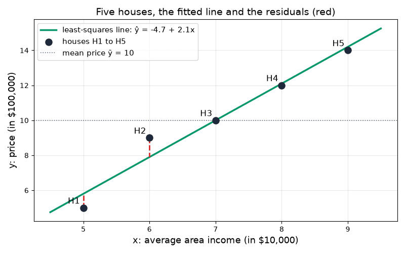
On a plot, the residual is the vertical distance from the point to the line

Least Squares

SSE = ∑ (y_i − ŷ_i)²

SSE: the sum of squared errors over all n points
The least-squares line is the line with the smallest SSE
Squaring makes every error positive and punishes big errors more

b₁ = ∑ (x_i − x̄)(y_i − ȳ)∑ (x_i − x̄)²

b₀ = ȳ − b₁ x̄

By hand

Worked Example: Five Real Houses

Rows of USA_Housing.csv. x: income in $10,000, y: price in $100,000, rounded

House	Income	Price	(x, y)
H1	$50,016	$497,368	(5, 5)
H2	$59,769	$897,291	(6, 9)
H3	$69,529	$995,137	(7, 10)
H4	$79,628	$1,196,064	(8, 12)
H5	$89,548	$1,403,803	(9, 14)

Step 1: The Means

x̄ = 5 + 6 + 7 + 8 + 95 = 7

ȳ = 5 + 9 + 10 + 12 + 145 = 10

Step 2: Deviations from the Means

House	(x − x̄, y − ȳ)	Product	(x − x̄)²
H1	(-2, -5)	10	4
H2	(-1, -1)	1	1
H3	(0, 0)	0	0
H4	(1, 2)	2	1
H5	(2, 4)	8	4

Step 3: Slope and Intercept

b₁ = 2110 = 2.1

b₀ = 10 − 2.1 × 7 = −4.7

Step 4: Predictions and Residuals

House	ŷ	e = y − ŷ	e²
H1	5.8	-0.8	0.64
H2	7.9	1.1	1.21
H3	10.0	0.0	0.00
H4	12.1	-0.1	0.01
H5	14.2	-0.2	0.04

Step 5: Is It Really the Best Line?

Line	SSE
ŷ = −3 + 2x	7.0
ŷ = −4 + 2x	2.0
ŷ = −4.7 + 2.1x	1.9

The five houses, the least-squares line and the residuals in red

Step 6: Predict a New Area

ŷ = −4.7 + 2.1 × 7.5 = 11.05

Try It: Least Squares, Live

Measuring the Error of a Line

MAE = 1n ∑ |e_i|

MSE = 1n ∑ e_i²

RMSE = √MSE

MAE: the average size of an error, in the units of y
MSE: the average squared error, in squared units
RMSE: back in the units of y, and big errors weigh more than in MAE

Worked Example: MAE, MSE, RMSE

MAE = 0.8 + 1.1 + 0 + 0.1 + 0.25 = 0.44

MSE = 1.905 = 0.38, RMSE = √0.38 = 0.6164

R²: Better Than the Mean?

R² = 1 − SSESST, SST = ∑ (y_i − ȳ)²

SST: the SSE of the flat line ŷ = ȳ, the best guess without a feature
R² = the share of that error the model removes: 1 is perfect, 0 is no better than the mean

SST = 25 + 1 + 0 + 4 + 16 = 46, R² = 1 − 1.9046 = 0.9587

Try It: What R² Measures

Part 2

Explore the Housing Data

The notebook, and the milestone of this week

Open the Notebook in Colab

text

https://colab.research.google.com/github/
tirthajyoti/Machine-Learning-with-Python/blob/
master/Regression/Linear_Regression_Practice.ipynb

Join the three lines into one address, or click "Open in Colab" on the lesson page.

Load and Inspect the Data

python

url = ("https://raw.githubusercontent.com/"
       "tirthajyoti/Machine-Learning-with-Python/"
       "master/Datasets/USA_Housing.csv")
df = pd.read_csv(url)
df.info(verbose=True)

5000 rows, 7 columns, all 5000 non-null: no missing values
Five numeric features and the target Price
Address is text: a linear model only multiplies numbers, so it stays out of X

The Distribution of the Price

python

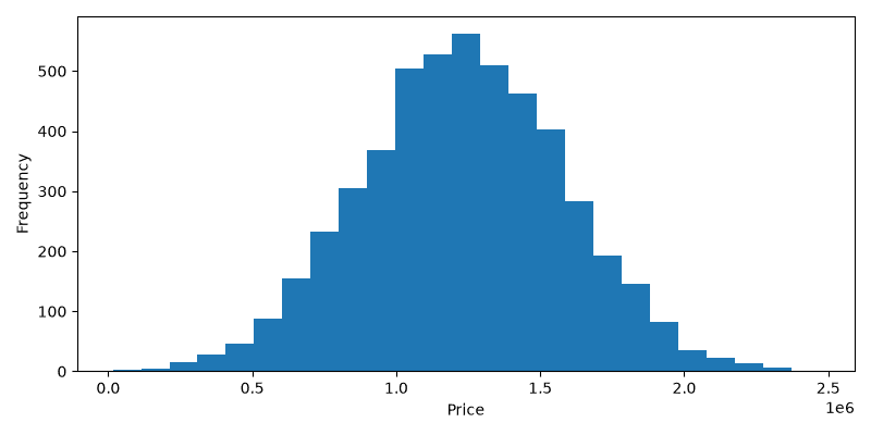
df['Price'].plot.hist(bins=25, figsize=(8,4))

One hill around the mean of about $1.23 million
Only 97 houses below $0.5 million and 74 above $2 million
1e6 under the axis: the ticks are in millions

Histogram of the 5000 house prices with 25 bins

Correlations with the Price

python

df.corr(numeric_only=True)

sns.heatmap(df.corr(numeric_only=True),
            annot=True, linewidths=2)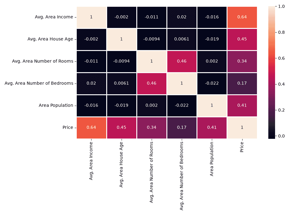

Correlation heatmap of the six numeric columns

Reading the Price Row

Feature	Correlation with Price
Avg. Area Income	0.640
Avg. Area House Age	0.453
Area Population	0.409
Avg. Area Number of Rooms	0.336
Avg. Area Number of Bedrooms	0.171

Part 3

Fit the Model

LinearRegression in scikit-learn

Features, Target, and the Split

python

X = df[l_column[0:len_feature-2]]   # 5 features
y = df[l_column[len_feature-2]]     # Price

from sklearn.model_selection import train_test_split
X_train, X_test, y_train, y_test = train_test_split(
    X, y, test_size=0.3, random_state=123)

The notebook imports from sklearn.cross_validation, which no longer exists: use sklearn.model_selection.

Fit and Read the Coefficients

python

lm = LinearRegression()
lm.fit(X_train, y_train)
print(lm.intercept_)

cdf = pd.DataFrame(data=lm.coef_,
    index=X_train.columns,
    columns=['Coefficients'])

Feature	Coefficient
Income	21.597602
House age	165201.104954
Rooms	119061.463868
Bedrooms	3212.585606
Population	15.228121

Reading a Coefficient

A coefficient is the change in ŷ when its feature grows by 1 and the others stay the same

Worked Example: One Test House by Hand

Row 2648, the first test house. Real price: $800,146.23

Feature	x	b × x
Income	63824.394539	1,378,453.87
House age	4.991750	824,642.62
Rooms	5.003836	595,764.04
Bedrooms	4.00	12,850.34
Population	40086.458749	610,441.44

Worked Example: Add the Intercept

ŷ = −2,631,028.90 + 3,422,152.31 = 791,123.41

e = 800,146.23 − 791,123.41 = 9,022.82

Which Features Matter Most?

The notebook divides each coefficient by its standard error: the t-statistic

Feature	t-statistic
Avg. Area Income	134.68
Avg. Area House Age	95.91
Area Population	89.64
Avg. Area Number of Rooms	70.18
Avg. Area Number of Bedrooms	2.33

Part 4

Evaluate the Model

Predict the 1500 test houses

Actual Against Predicted

python

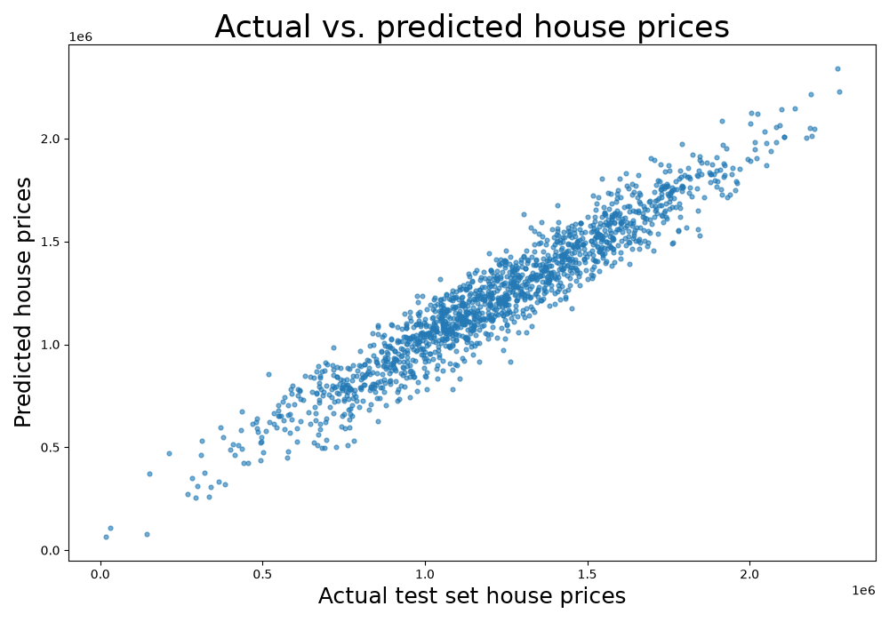
predictions = lm.predict(X_test)

plt.scatter(x=y_test, y=predictions)

predictions: 1500 prices, one per test house
A perfect model puts every point on the 45 degree line
The points form a narrow band along it, for cheap and expensive houses alike

Scatter of actual against predicted prices for the 1500 test houses

Checking the Residuals: the Histogram

Histogram of the test residuals with a density curve

Checking the Residuals: Against the Predictions

Residuals plotted against the predicted prices

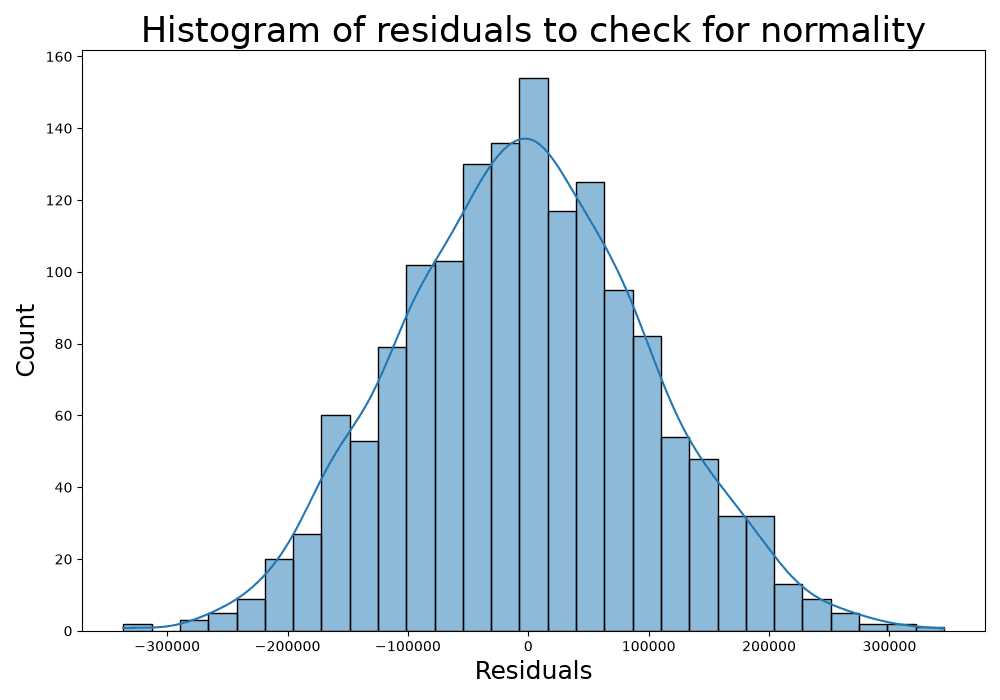
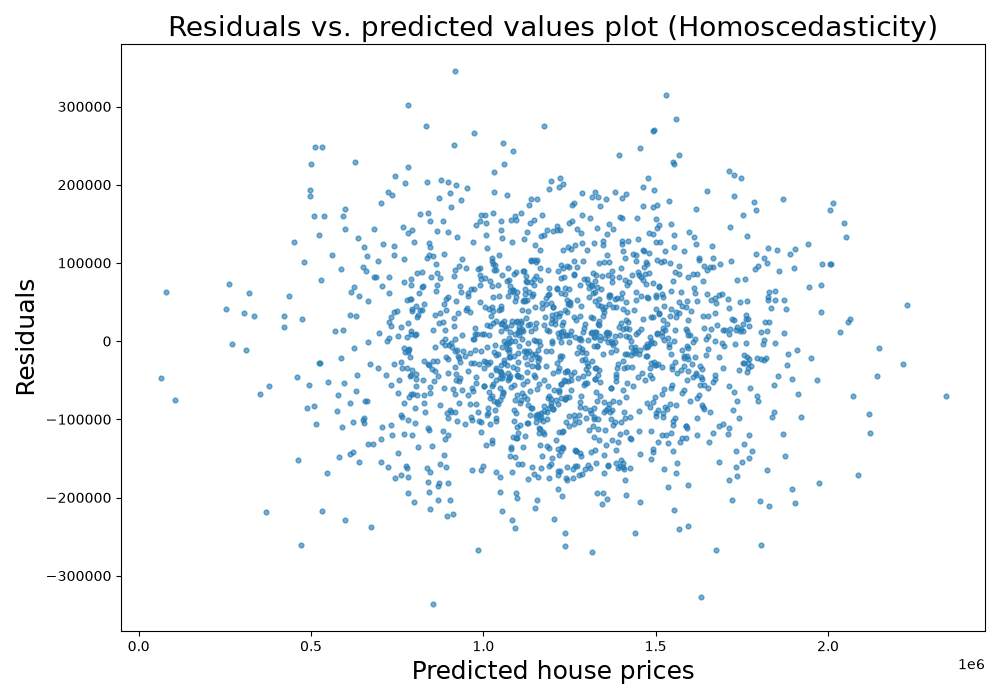
The Error Measures

text

Mean absolute error (MAE): 81739.77482718184
Mean square error (MSE): 10489638335.804983
Root mean square error (RMSE): 102418.93543581179
R-squared value of predictions: 0.919

RMSE = √10,489,638,335.80 = 102,418.94

Reading the Numbers

Measure	Value	Meaning
MAE	$81,740	average size of an error
RMSE	$102,419	typical error, about 8% of the mean price
Test R²	0.919	about 92% of the price spread explained
Training R²	0.917	as good on new houses as on seen ones

Before you practise

Common Mistakes

Running the old calls as they are: cross_validation, df.corr() with a text column, distplot
Reading ./Datasets/USA_Housing.csv in Colab
Leaving the text column Address in X
Ranking features by coefficient size when their units differ
Reporting only the training R²
Trusting a prediction far outside the training data, like the intercept at income 0

Your team project

Project Milestone: Explore and Clean Your Data

Check shape, the columns and the types with info()
Count missing values with isnull().sum(), then fillna or dropna (week 1)
Run describe() and look for impossible values
Plot the target as a histogram, and each feature against it
Draw the correlation heatmap with numeric_only=True
Drop columns a model cannot use, such as free text or IDs

Part 5

Practice: Your Turn

About 30 minutes, answers follow each task

About 10 minutes

Practice 1: Fit a Line by Hand

Area	x (income, $10,000)	y (price, $100,000)
A1	4	6
A2	5	7
A3	6	10
A4	7	11
A5	8	11

Compute x̄, ȳ, the slope b₁ and the intercept b₀
Compute the residuals, SSE, MSE, RMSE, MAE and R²
Predict the price for an income of $65,000

Answers

Practice 1: Answer, the Line

b₁ = 6 + 2 + 0 + 2 + 44 + 1 + 0 + 1 + 4 = 1410 = 1.4

b₀ = ȳ − b₁ x̄ = 9 − 1.4 × 6 = 0.6

Answers

Practice 1: Answer, the Error

Area	ŷ	e	e²
A1	6.2	-0.2	0.04
A2	7.6	-0.6	0.36
A3	9.0	1.0	1.00
A4	10.4	0.6	0.36
A5	11.8	-0.8	0.64

SSE = 2.40, MSE = 0.48, RMSE = 0.6928

MAE = 0.64, SST = 22, R² = 1 − 2.4022 = 0.8909

About 5 minutes

Practice 2: A Second Test House

Row 2456, real price $707,345.06, intercept -2,631,028.90. Predict, then find the residual.

Feature	x	Coefficient b
Income	67041.967661	21.597602
House age	6.021458	165201.104954
Rooms	5.346830	119061.463868
Bedrooms	3.39	3212.585606
Population	15633.099048	15.228121

Answers

Practice 2: Answer

ŷ = −2,631,028.90 + 3,328,252.05 = 697,223.15

About 5 minutes

Practice 3: Read the Coefficients

Two areas differ only by 2 years of house age. How far apart are the predictions?
They differ only by $5,000 of income. How far apart now?
Why does the bedrooms coefficient, 3212.59, not mean bedrooms matter more than income?

2 × 165,201.10 ≈ 330,402, 5,000 × 21.597602 ≈ 107,988

About 10 minutes

Practice 4: In Colab

Run the notebook with the three fixes of today, up to the error measures
Fit lm1 on X_train[['Avg. Area Income']] only: print intercept, coefficient, test R², MAE, RMSE
Fit a model on all features except Avg. Area Number of Bedrooms (drop(..., axis=1)) and print its test R²
Compare the three R² values: what do they say about the features?

Answers

Practice 4: Answer

Model	Test R²	Test RMSE
All five features	0.919	102,418.94
Income only	0.417	275,407.48
All except bedrooms	0.920	102,282.54

Key Takeaways

Linear regression predicts a number as b0 plus a weighted sum of the features
A residual is y − ŷ; least squares makes the sum of their squares smallest
Explore and clean first: types, missing values, text columns, correlations
A coefficient is the change per unit of its feature: rank features by t-statistic
Judge the model on the test set with MAE, RMSE, R² and the residual plots

Open this lesson

Mahmoud AbasLinear Regression

Part

What we do

Time

The idea, least squares, a worked example by hand

35 min

Notebook: explore and prepare the housing data

20 min

Notebook: fit the model, read the coefficients

20 min

Evaluate on the test set, your project

15 min

Practice with answers, then takeaways

30 min

House

Income

Price

(x, y)

$50,016

$497,368

(5, 5)

$59,769

$897,291

(6, 9)

$69,529

$995,137

(7, 10)

$79,628

$1,196,064

(8, 12)

$89,548

$1,403,803

(9, 14)

House

(x − x̄, y − ȳ)

Product

(x − x̄)²

(-2, -5)

(-1, -1)

(0, 0)

(1, 2)

(2, 4)

House

e = y − ŷ

e²

5.8

-0.8

0.64

7.9

1.1

1.21

10.0

0.0

0.00

12.1

-0.1

0.01

14.2

-0.2

0.04

Line

SSE

ŷ = −3 + 2x

7.0

ŷ = −4 + 2x

2.0

ŷ = −4.7 + 2.1x

1.9

Feature

Correlation with Price

Avg. Area Income

0.640

Avg. Area House Age

0.453

Area Population

0.409

Avg. Area Number of Rooms

0.336

Avg. Area Number of Bedrooms

0.171

X = df[l_column[0:len_feature-2]] # 5 features y = df[l_column[len_feature-2]] # Price from sklearn.model_selection import train_test_split X_train, X_test, y_train, y_test = train_test_split( X, y, test_size=0.3, random_state=123)

Feature

Coefficient

Income

21.597602

House age

165201.104954

Rooms

119061.463868

Bedrooms

3212.585606

Population

15.228121

Feature

b × x

Income

63824.394539

1,378,453.87

House age

4.991750

824,642.62

Rooms

5.003836

595,764.04

Bedrooms

4.00

12,850.34

Population

40086.458749

610,441.44

Feature

t-statistic

Avg. Area Income

134.68

Avg. Area House Age

95.91

Area Population

89.64

Avg. Area Number of Rooms

70.18

Avg. Area Number of Bedrooms

2.33

Measure

Value

Meaning

MAE

$81,740

average size of an error

RMSE

$102,419

typical error, about 8% of the mean price

Test R²

0.919

about 92% of the price spread explained

Training R²

0.917

as good on new houses as on seen ones

Area

x (income, $10,000)

y (price, $100,000)

Area

e²

6.2

-0.2

0.04

7.6

-0.6

0.36

9.0

1.0

1.00

10.4

0.6

0.36

11.8

-0.8

0.64

Feature

Coefficient b

Income

67041.967661

21.597602

House age

6.021458

165201.104954

Rooms

5.346830

119061.463868

Bedrooms

3.39

3212.585606

Population

15633.099048

15.228121

Model

Test R²

Test RMSE

All five features

0.919

102,418.94

Income only

0.417

275,407.48

All except bedrooms

0.920

102,282.54