

k-Means Clustering
Every model so far in this course learned from labelled rows: a price, a class, spam or ham. This section starts unsupervised learning, where the rows carry no label at all. k-means groups similar rows into k clusters on its own. You will run the algorithm by hand on five real customers, then use the two notebooks of week 8 to segment 200 mall customers for a marketing campaign and to group 777 colleges without telling the model which ones are private.
Objectives
By the end of the section you should be able to:
- Explain the difference between supervised learning and clustering.
- Run k-means by hand: assign every point to its nearest centroid, move every centroid to the mean of its points, and repeat until nothing changes.
- Compute the within-cluster sum of squares (WCSS), which scikit-learn calls
inertia_. - Fit
KMeans, readcluster_centers_,labels_andpredict, and choose k with the elbow method. - Segment customers and decide which segment a campaign should target.
- Explain why a different start can give a different result, and what
n_initdoes about it.
Where this sits in the course
Week 8 of the plan has three parts:
- Two notebooks.
Clusteringgroups generated points and then real customer data.K_Means_Clustering_Practicegroups 777 US colleges into two clusters and compares them with the real private and public labels. - A real-world scenario. Segmenting customers based on customer data to identify which customers to target with a campaign for a new product or a promotion to increase their purchasing activity.
- A project milestone. Project Teams Presentations and Discussions: this week your team presents its project and discusses it.
In week 5 you measured Euclidean distances for KNN, and in weeks 3 to 7 you called fit and predict on many models. k-means uses both: the same distance, and the same fit and predict pattern. What is new is that there is no y to learn from.
| Part | What we do | Time |
|---|---|---|
| 1 | Clustering and the k-means algorithm, then five customers by hand | 40 min |
| 2 | Notebook 1: blobs and the elbow method | 15 min |
| 3 | Notebook 1: segmenting customers | 20 min |
| 4 | Notebook 2: colleges, and the project milestone | 15 min |
| 5 | Practice with answers, then takeaways | 30 min |
Part 1: The idea of clustering
Supervised learning and clustering
| Supervised (weeks 3 to 7) | Clustering (this week) | |
|---|---|---|
| Training data | features X and a label y | features X only |
| What the model learns | how to predict y | groups of similar rows |
| Example | KNN predicts the iris species | k-means finds customer segments |
| Checking the result | compare predictions with the true y | usually no true answer exists |
Clustering is an unsupervised learning method for grouping data into clusters to detect similarities. k-means is a popular method for performing clustering, and scikit-learn implements it in the KMeans class.
What k-means is
The k-means algorithm divides a set of samples into k clusters that do not overlap. Each cluster is described by the mean of its samples, called its centroid. A centroid is usually not one of the data points, but it lives in the same space: for customers described by income and spending, a centroid is also an (income, spending) pair.
The algorithm
- Choose k and place k starting centroids, for example on k points picked at random from the data.
- Assign step: every point joins the cluster of its nearest centroid, measured with the squared Euclidean distance.
- Update step: every centroid moves to the mean of the points assigned to it.
- Repeat steps 2 and 3 until no point changes its cluster (or a maximum number of iterations is reached).
The algorithm is guaranteed to stop. The result can be a local optimum, not necessarily the best possible grouping, so it is worth running it several times from different random starts and keeping the best run.
The formulas
For a point (x, y) and a centroid (a, b), the squared distance is:
The square root is not needed: it never changes which centroid is nearest.
In the update step, a cluster with points moves its centroid to:
How good is a clustering? WCSS
Add up the squared distance from every point to the centroid of its own cluster:
Here N is the number of points and is the distance from point to its own centroid. J is the within-cluster sum of squares (WCSS). scikit-learn calls it inertia and stores it in kmeans.inertia_. A small J means tight clusters, points close to their centroids. The k-means algorithm is built to make J small.
Worked example: five customers by hand
We take five real customers from the customer dataset of notebook 1, with two features: annual income in thousands of dollars, and a spending score from 1 to 100.
| Customer | Income (k$) | Spending score |
|---|---|---|
| #11 | 19 | 14 |
| #49 | 40 | 42 |
| #62 | 46 | 55 |
| #136 | 73 | 88 |
| #190 | 103 | 85 |
We use k = 2, and start the two centroids on two of the customers: μ1 = #11 = (19, 14) and μ2 = #62 = (46, 55). Each difference below is customer minus centroid, and a negative difference squares to a positive number.
Iteration 1: assign
| Customer | (income, spending) | d² to μ1 (19, 14) | d² to μ2 (46, 55) | Joins |
|---|---|---|---|---|
| #11 | (19, 14) | 0 + 0 = 0 | 729 + 1681 = 2410 | μ1 |
| #49 | (40, 42) | 441 + 784 = 1225 | 36 + 169 = 205 | μ2 |
| #62 | (46, 55) | 729 + 1681 = 2410 | 0 + 0 = 0 | μ2 |
| #136 | (73, 88) | 2916 + 5476 = 8392 | 729 + 1089 = 1818 | μ2 |
| #190 | (103, 85) | 7056 + 5041 = 12097 | 3249 + 900 = 4149 | μ2 |
For #49, for example: (40 - 19)² + (42 - 14)² = 441 + 784 = 1225 and (40 - 46)² + (42 - 55)² = 36 + 169 = 205, so #49 joins μ2.
Cluster 1 holds only #11. Cluster 2 holds the other four.
Iteration 1: update
- μ1 has one point, so it stays at (19, 14).
- μ2 moves to the mean of #49, #62, #136 and #190: income
(40 + 46 + 73 + 103) / 4 = 262 / 4 = 65.5, spending(42 + 55 + 88 + 85) / 4 = 270 / 4 = 67.5, so μ2 = (65.5, 67.5).
Iteration 2: assign
| Customer | (income, spending) | d² to μ1 (19, 14) | d² to μ2 (65.5, 67.5) | Joins |
|---|---|---|---|---|
| #11 | (19, 14) | 0 + 0 = 0 | 2162.25 + 2862.25 = 5024.5 | μ1 |
| #49 | (40, 42) | 441 + 784 = 1225 | 650.25 + 650.25 = 1300.5 | μ1 |
| #62 | (46, 55) | 729 + 1681 = 2410 | 380.25 + 156.25 = 536.5 | μ2 |
| #136 | (73, 88) | 2916 + 5476 = 8392 | 56.25 + 420.25 = 476.5 | μ2 |
| #190 | (103, 85) | 7056 + 5041 = 12097 | 1406.25 + 306.25 = 1712.5 | μ2 |
#49 changes cluster. The centroid μ2 moved away toward the rich, high-spending customers, and now #49 is a little closer to μ1 (1225 against 1300.5).
Iteration 2: update
- μ1 = mean of #11 and #49:
(19 + 40) / 2 = 29.5and(14 + 42) / 2 = 28, so μ1 = (29.5, 28). - μ2 = mean of #62, #136 and #190:
(46 + 73 + 103) / 3 = 222 / 3 = 74and(55 + 88 + 85) / 3 = 228 / 3 = 76, so μ2 = (74, 76).
Iteration 3: assign
| Customer | (income, spending) | d² to μ1 (29.5, 28) | d² to μ2 (74, 76) | Joins |
|---|---|---|---|---|
| #11 | (19, 14) | 110.25 + 196 = 306.25 | 3025 + 3844 = 6869 | μ1 |
| #49 | (40, 42) | 110.25 + 196 = 306.25 | 1156 + 1156 = 2312 | μ1 |
| #62 | (46, 55) | 272.25 + 729 = 1001.25 | 784 + 441 = 1225 | μ1 |
| #136 | (73, 88) | 1892.25 + 3600 = 5492.25 | 1 + 144 = 145 | μ2 |
| #190 | (103, 85) | 5402.25 + 3249 = 8651.25 | 841 + 81 = 922 | μ2 |
#62 changes cluster too (1001.25 against 1225).
Iteration 3: update
- μ1 = mean of #11, #49 and #62:
(19 + 40 + 46) / 3 = 105 / 3 = 35and(14 + 42 + 55) / 3 = 111 / 3 = 37, so μ1 = (35, 37). - μ2 = mean of #136 and #190:
(73 + 103) / 2 = 88and(88 + 85) / 2 = 86.5, so μ2 = (88, 86.5).
Iteration 4: assign, and stop
| Customer | (income, spending) | d² to μ1 (35, 37) | d² to μ2 (88, 86.5) | Joins |
|---|---|---|---|---|
| #11 | (19, 14) | 256 + 529 = 785 | 4761 + 5256.25 = 10017.25 | μ1 |
| #49 | (40, 42) | 25 + 25 = 50 | 2304 + 1980.25 = 4284.25 | μ1 |
| #62 | (46, 55) | 121 + 324 = 445 | 1764 + 992.25 = 2756.25 | μ1 |
| #136 | (73, 88) | 1444 + 2601 = 4045 | 225 + 2.25 = 227.25 | μ2 |
| #190 | (103, 85) | 4624 + 2304 = 6928 | 225 + 2.25 = 227.25 | μ2 |
No customer changes cluster, so the centroids would not move again: the algorithm has converged. The final clusters are (#11, #49, #62) around (35, 37), customers with lower income and lower spending, and (#136, #190) around (88, 86.5), customers with high income and high spending.
WCSS never went up
After every step we can add the squared distances of the five customers to their own centroid (the bold numbers of the cluster each customer is in):
| Iteration | J after the assign step | J after the update step |
|---|---|---|
| 1 | 0 + 205 + 0 + 1818 + 4149 = 6172 | 4026 |
| 2 | 0 + 1225 + 536.5 + 476.5 + 1712.5 = 3950.5 | 2904.5 |
| 3 | 306.25 + 306.25 + 1001.25 + 145 + 922 = 2680.75 | 1734.5 |
| 4 | 785 + 50 + 445 + 227.25 + 227.25 = 1734.5 | converged |
Both steps lower J or leave it the same: the assign step gives every point its nearest centroid, and in the update step the mean is the position with the smallest total squared distance to the points of its cluster. The final J = 1734.5 is exactly what scikit-learn reports. We checked it with KMeans(n_clusters=2, init=start, n_init=1), where start holds the two starting centroids:
import numpy as np
from sklearn.cluster import KMeans

X = np.array([[19, 14], [40, 42], [46, 55], [73, 88], [103, 85]])
start = np.array([[19, 14], [46, 55]])
kmeans = KMeans(n_clusters=2, init=start, n_init=1).fit(X)
print(kmeans.cluster_centers_)   # [[35.  37. ] [88.  86.5]]
print(kmeans.labels_)            # [0 0 0 1 1]
print(kmeans.inertia_)           # 1734.5
scikit-learn numbers the clusters from 0, so its cluster 0 is our μ1.
Open the k-means animator full screen to replay this example one step at a time. Drag a centroid to try another start, raise k, or switch to all 200 customers or to your own points.
Part 2: Notebook 1, blobs and the elbow method
Open the notebook
The outputs on this page come from scikit-learn 1.9.1. Colab may run another version, and then the cluster numbers, or even the clusters found from a single start, can differ from the ones shown here.
Generate four blobs
from sklearn.cluster import KMeans
from sklearn.datasets import make_blobs

import numpy as np
import matplotlib.pyplot as plt
import seaborn as sns

sns.set()

points, cluster_indexes = make_blobs(n_samples=300, centers=4, cluster_std=0.8, random_state=0)

x = points[:, 0]
y = points[:, 1]

plt.scatter(x, y, s=50, alpha=0.7)
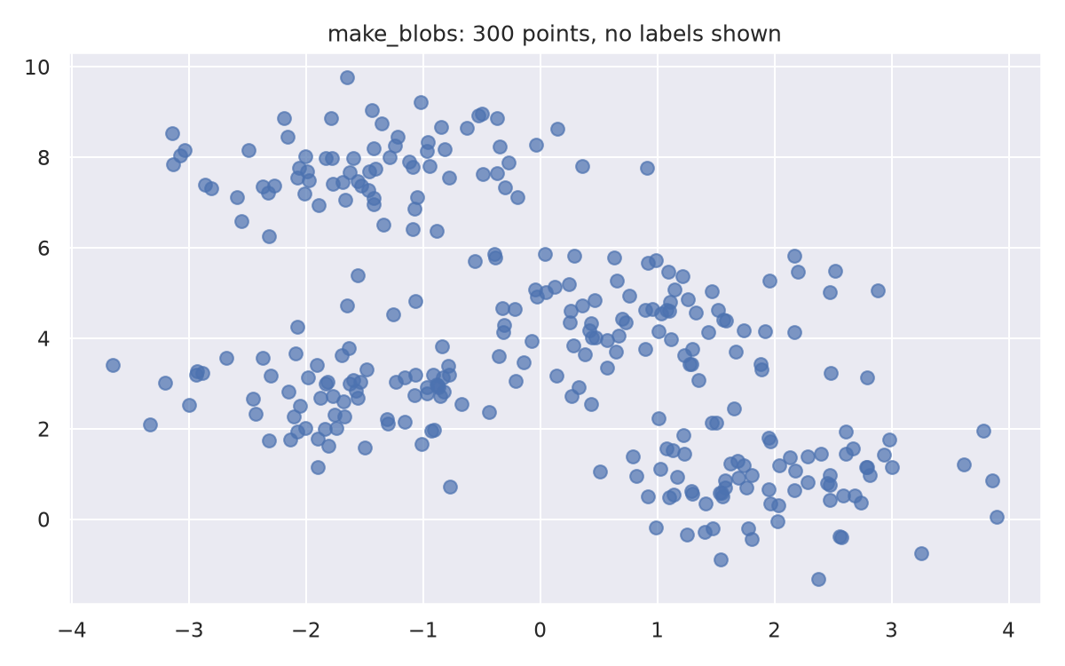
make_blobs generates 300 points loosely grouped into four clusters of 75 points each. The plot shows them without any colour: k-means never sees cluster_indexes.
Try three values of k
kmeans = KMeans(n_clusters=4, random_state=0)
kmeans.fit(points)
predicted_cluster_indexes = kmeans.predict(points)

plt.scatter(x, y, c=predicted_cluster_indexes, s=50, alpha=0.7, cmap='viridis')

centers = kmeans.cluster_centers_
plt.scatter(centers[:, 0], centers[:, 1], c='red', s=100)
The notebook runs this cell with n_clusters set to 3, 4 and 5. The red dots are the centroids.
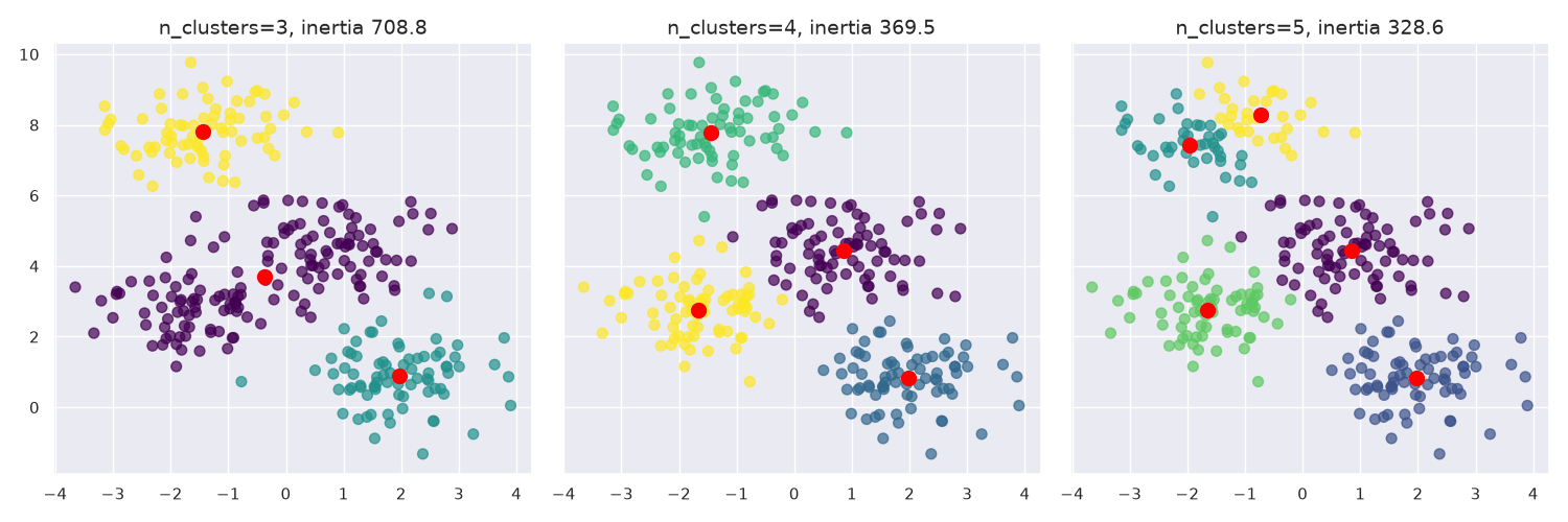
- k = 3 merges two blobs into one big cluster of 151 points. Inertia 708.77.
- k = 4 finds the four blobs: 81, 74, 73 and 72 points. Inertia 369.53.
- k = 5 cuts one real blob into two clusters of 42 and 31 points. Inertia 328.65.
k-means always returns exactly the k clusters you ask for, even when the data has a different number of groups.
Which cluster does a new point belong to?
The notebook adds the point (-0.5, 5), predicts its cluster with the k = 4 model, and then prints its distance to each of the four centroids:
point = np.array([[-0.5, 5]])
px = point[:, 0]
py = point[:, 1]

cluster = kmeans.predict(point)[0]
print(cluster)

d = []
for i in range(len(centers)):
    d.append(np.sqrt((px - centers[i][0])**2 + (py - centers[i][1])**2))

print(d)
0
[array([1.46570934]), array([4.8470332]), array([2.93542029]), array([2.52147763])]The smallest distance, 1.466, is to centroid 0 at (0.85, 4.44), so the point joins cluster 0. predict does exactly the assign step of the algorithm.
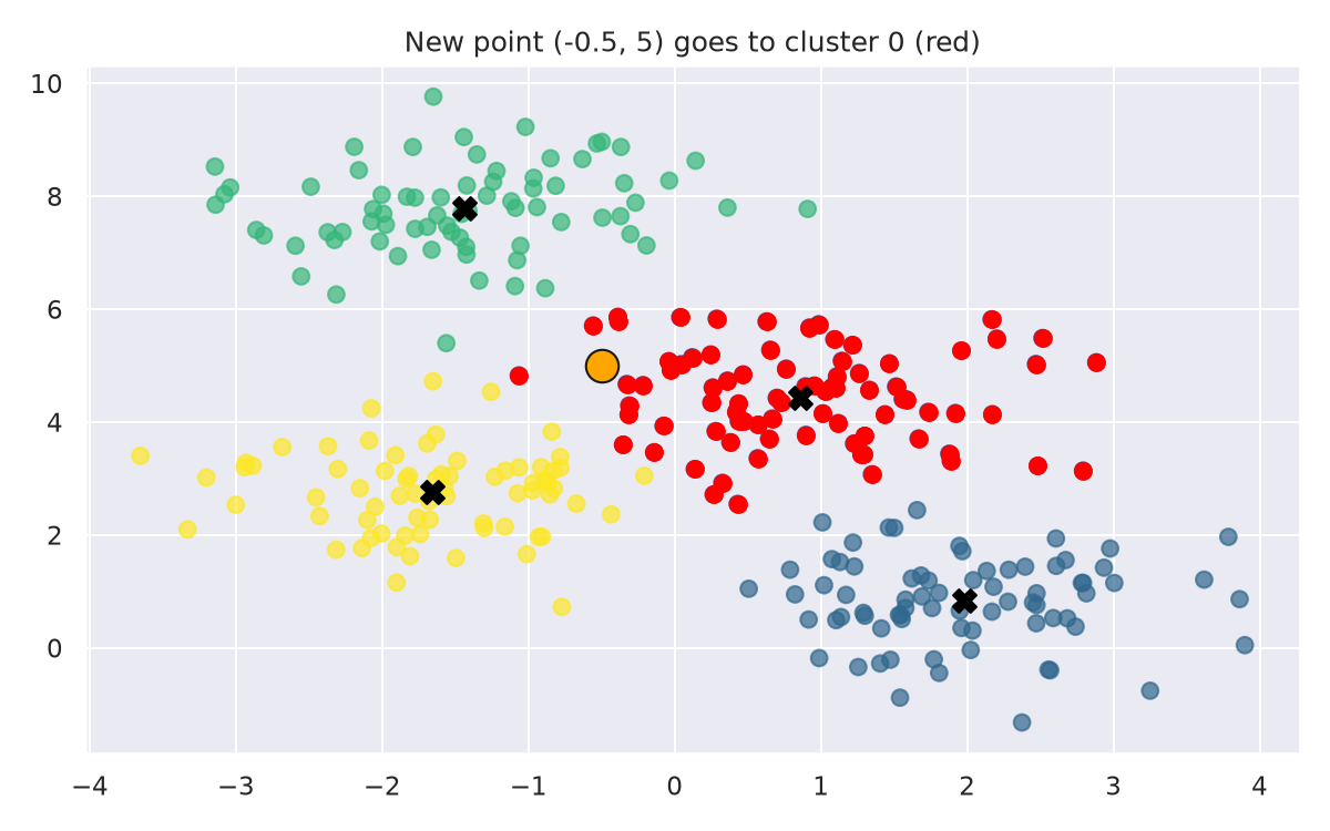
The saved notebook printed 1 for the same point, with the same four distances in a different order. The cluster numbers are only names: which group is called 0 depends on the run.
Choosing k: the elbow method
inertias = []

for i in range(1, 10):
    kmeans = KMeans(n_clusters=i, random_state=0)
    kmeans.fit(points)
    inertias.append(kmeans.inertia_)

plt.plot(range(1, 10), inertias)
plt.xlabel('Number of Clusters')
plt.ylabel('Inertia')| k | Inertia | Drop from k - 1 |
|---|---|---|
| 1 | 2978.59 | |
| 2 | 1351.37 | 1627.22 |
| 3 | 708.77 | 642.60 |
| 4 | 369.53 | 339.24 |
| 5 | 328.65 | 40.88 |
| 6 | 298.52 | 30.13 |
| 7 | 267.07 | 31.45 |
| 8 | 232.65 | 34.42 |
| 9 | 211.99 | 20.66 |
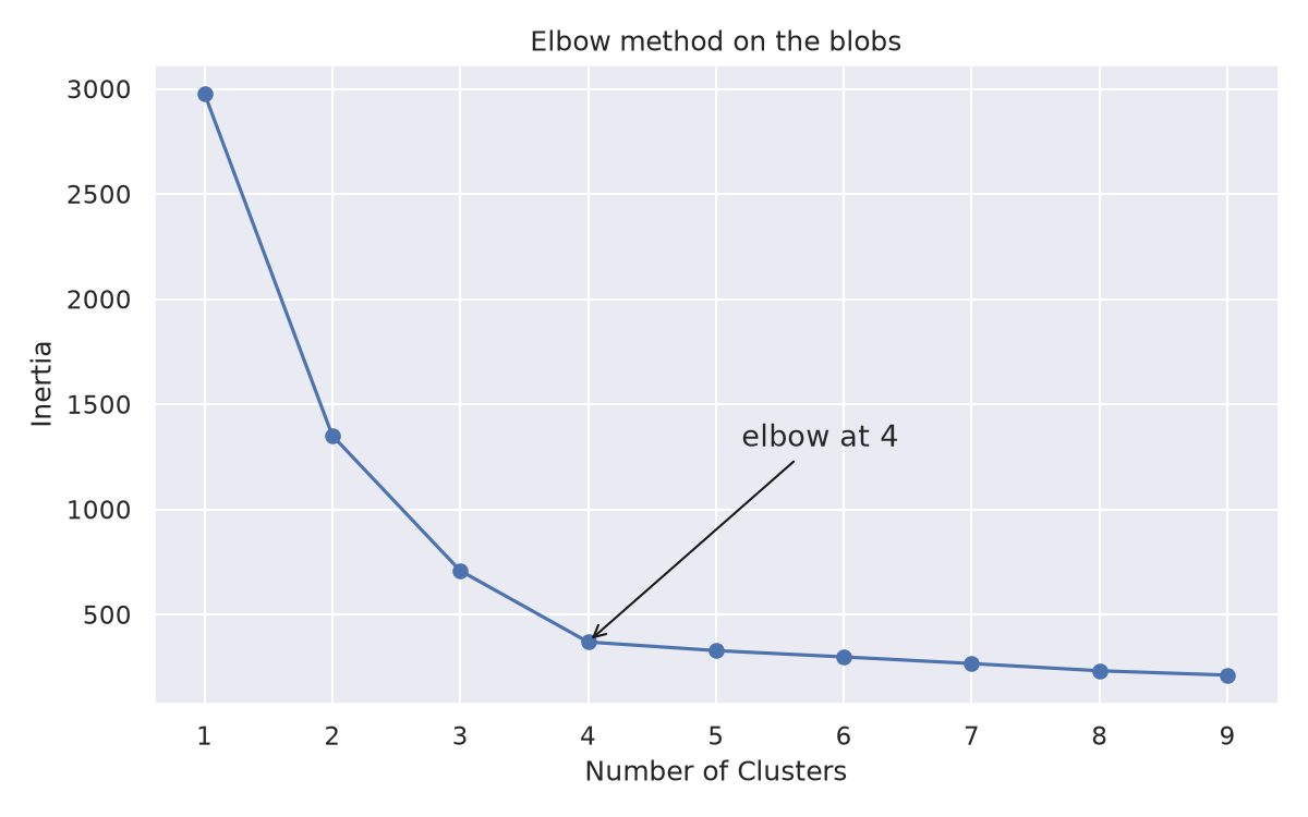
- Inertia always falls as k grows: with more centroids every point can be closer to one. With k equal to the number of points it would be 0.
- So do not pick the k with the smallest inertia. Pick the elbow: the k after which the drops become small. Here the drop from 3 to 4 is 339.24 and the drop from 4 to 5 is only 40.88, so k = 4, the number of blobs that were generated.
Open the elbow method widget full screen to replay the loop one k at a time and see the clusters behind every point on the curve.
Part 3: Segmenting customers
The scenario
A mall wants to launch a campaign for a new product, or a promotion that makes customers buy more. It cannot send the same offer to everyone, so it segments its customers from their data and targets the right segment. The notebook uses a customer-segmentation dataset from Kaggle with 200 customers:
| Column | Meaning |
|---|---|
CustomerID | a number from 1 to 200 |
Gender | Male or Female (88 and 112 customers) |
Age | 18 to 70 |
Annual Income (k$) | 15 to 137 thousand dollars |
Spending Score (1-100) | 1 to 99, a score the mall gives to how much the customer spends |
Load the data
The notebook reads Data/customers.csv, a folder that does not exist when the notebook opens in Colab. Read the file from the repository instead:
import pandas as pd

url = ("https://raw.githubusercontent.com/"
       "jeffprosise/Machine-Learning/master/Data/customers.csv")
customers = pd.read_csv(url)
customers.head()
CustomerID Gender Age Annual Income (k$) Spending Score (1-100)
0 1 Male 19 15 39
1 2 Male 21 15 81
2 3 Female 20 16 6
3 4 Female 23 16 77
4 5 Female 31 17 40customers.shape is (200, 5), and customers.info() shows 200 non-null values in every column, so nothing is missing.
Two features: income and spending
points = customers.iloc[:, 3:5].values
x = points[:, 0]
y = points[:, 1]

plt.scatter(x, y, s=50, alpha=0.7)
plt.xlabel('Annual Income (k$)')
plt.ylabel('Spending Score')
iloc[:, 3:5] takes columns 3 and 4, the income and the spending score.
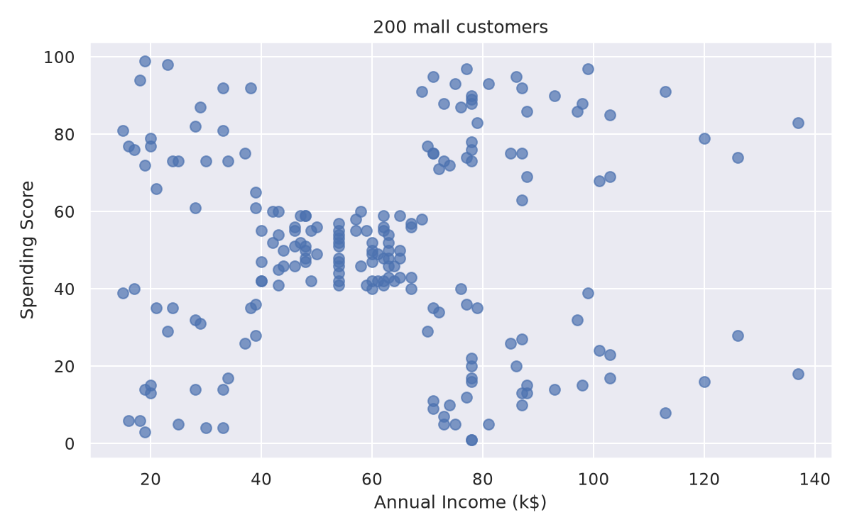
Even by eye you can see a dense group in the middle and four groups in the corners.
The elbow on the customers
The notebook runs the same elbow loop on points:
| k | 1 | 2 | 3 | 4 | 5 | 6 | 7 | 8 | 9 |
|---|---|---|---|---|---|---|---|---|---|
| Inertia | 269981.28 | 185917.14 | 106348.37 | 73679.79 | 44448.46 | 38858.96 | 31969.43 | 29858.48 | 22209.85 |
The drop from 4 to 5 is 29231.33; the drop from 5 to 6 is only 5589.50. The elbow is at k = 5.
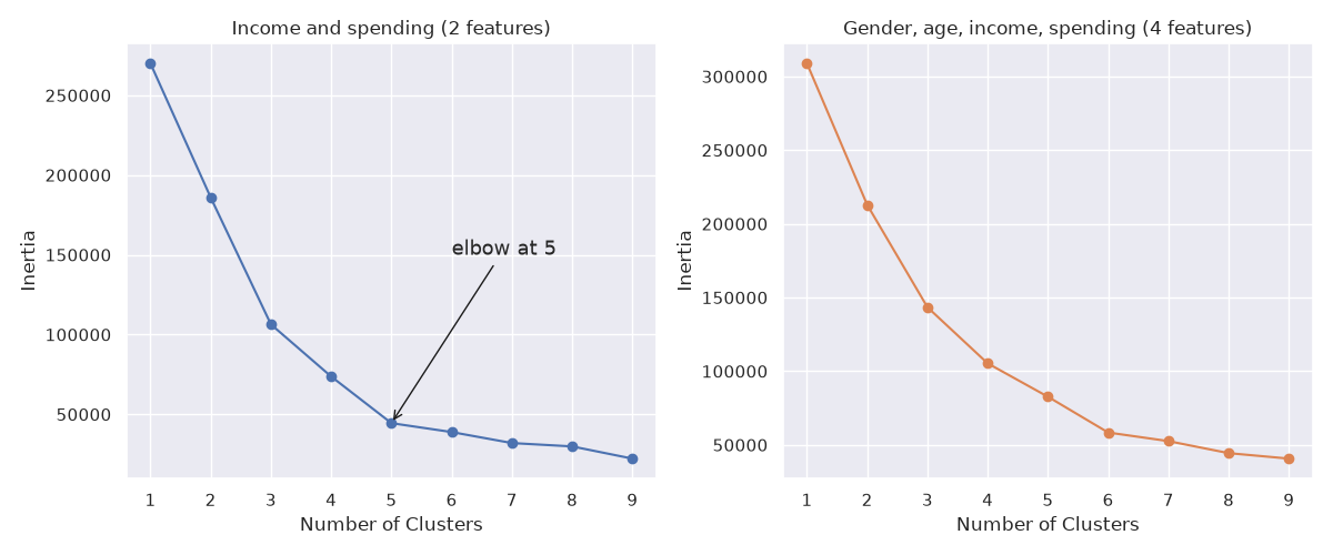
Five segments
kmeans = KMeans(n_clusters=5, random_state=0)
kmeans.fit(points)
predicted_cluster_indexes = kmeans.predict(points)

plt.scatter(x, y, c=predicted_cluster_indexes, s=50, alpha=0.7, cmap='viridis')
plt.xlabel('Annual Income (k$)')
plt.ylabel('Spending Score')

centers = kmeans.cluster_centers_
plt.scatter(centers[:, 0], centers[:, 1], c='red', s=100)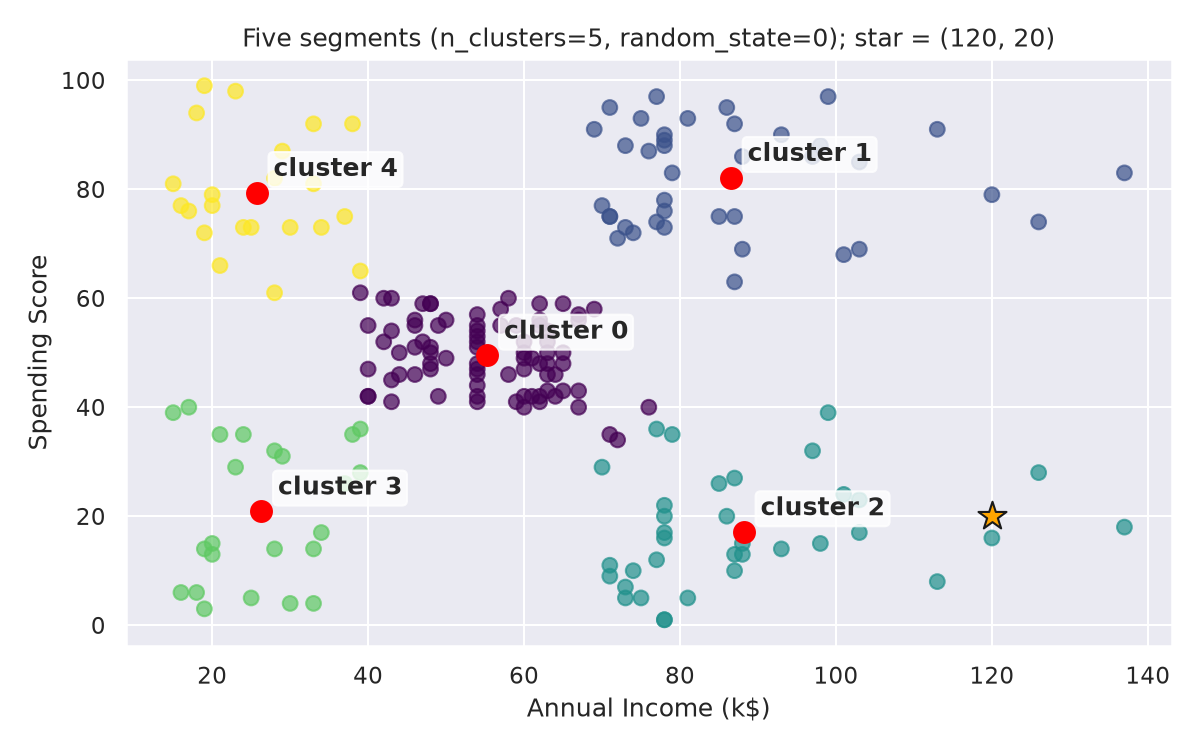
Each centroid is the average customer of its segment:
| Cluster | Average income (k$) | Average spending | Customers | A name for the segment |
|---|---|---|---|---|
| 0 | 55.30 | 49.52 | 81 | average income, average spending |
| 1 | 86.54 | 82.13 | 39 | high income, high spending |
| 2 | 88.20 | 17.11 | 35 | high income, low spending |
| 3 | 26.30 | 20.91 | 23 | low income, low spending |
| 4 | 25.73 | 79.36 | 22 | low income, high spending |
The names are ours. k-means only returns numbers; a person reads the centroids and decides what each segment means.
Which customers to target?
A promotion to increase purchasing activity should reach customers who can spend more but do not: high income, low spending. The notebook finds their cluster by predicting a made-up customer with an income of 120 and a spending score of 20, then lists every customer in that cluster:
df = customers.copy()
df['Cluster'] = kmeans.predict(points)

cluster = kmeans.predict(np.array([[120, 20]]))[0]
clustered_df = df[df['Cluster'] == cluster]
clustered_df['CustomerID'].values
array([125, 129, 131, 135, 137, 139, 141, 145, 147, 149, 151, 153, 155,
157, 159, 161, 163, 165, 167, 169, 171, 173, 175, 177, 179, 181,
183, 185, 187, 189, 191, 193, 195, 197, 199])The made-up customer falls in cluster 2, and the campaign list holds its 35 customers. For a loyalty program that rewards customers who already buy a lot, you would pick the high-spending segments instead: cluster 1, and possibly cluster 4.
Segment on all attributes
The notebook then clusters on gender, age, income and spending. KMeans needs numbers, so it first replaces the strings Female and Male with 0 and 1, which is called label encoding:
from sklearn.preprocessing import LabelEncoder

df = customers.copy()
encoder = LabelEncoder()
df['Gender'] = encoder.fit_transform(df['Gender'])
points = df.iloc[:, 1:5].values
encoder.classes_ is ['Female' 'Male'], so Female becomes 0 and Male becomes 1. iloc[:, 1:5] takes the four columns from Gender to the spending score and leaves out CustomerID, which is only a row number.
The elbow loop gives:
| k | 1 | 2 | 3 | 4 | 5 | 6 | 7 | 8 | 9 |
|---|---|---|---|---|---|---|---|---|---|
| Inertia | 308862.06 | 212889.44 | 143391.59 | 105299.99 | 82657.05 | 58387.21 | 52544.81 | 44389.81 | 40670.99 |
The elbow is less distinct this time. The notebook keeps five clusters and reports each one:
kmeans = KMeans(n_clusters=5, random_state=0)
kmeans.fit(points)
df['Cluster'] = kmeans.predict(points)

results = pd.DataFrame(columns = ['Cluster', 'Average Age', 'Average Income', 'Average Spending Index', 'Number of Females', 'Number of Males'])

for i in range(len(kmeans.cluster_centers_)):
    age = df[df['Cluster'] == i]['Age'].mean()
    income = df[df['Cluster'] == i]['Annual Income (k$)'].mean()
    spend = df[df['Cluster'] == i]['Spending Score (1-100)'].mean()

    gdf = df[df['Cluster'] == i]
    females = gdf[gdf['Gender'] == 0].shape[0]
    males = gdf[gdf['Gender'] == 1].shape[0]

    results.loc[i] = ([i, age, income, spend, females, males])

results.head()| Cluster | Average age | Average income | Average spending | Females | Males |
|---|---|---|---|---|---|
| 0 | 54.06 | 40.46 | 36.72 | 28 | 22 |
| 1 | 32.69 | 86.54 | 82.13 | 21 | 18 |
| 2 | 25.25 | 25.83 | 76.92 | 14 | 10 |
| 3 | 41.65 | 88.74 | 16.76 | 15 | 19 |
| 4 | 33.40 | 58.06 | 48.77 | 34 | 19 |
The high-income, low-spending segment is cluster 3 here: 34 customers, average age 41.65, 15 women and 19 men. The notebook asks whether it would matter to target men or women: this segment holds both in similar numbers, so for this promotion income and spending decide the target, not gender.
A different start, a different result
The saved notebook shows a different table for the same cell: average ages 45.22, 32.69, 43.09, 40.67 and 25.52. The reason is the start.
KMeansplaces its starting centroids with a random method (init='k-means++') controlled byrandom_state.n_initis how many times it runs the whole algorithm from different starts; it keeps the run with the smallest inertia.- Since scikit-learn 1.4 the default is
n_init='auto', which fork-means++means one run.
Run the same cell with n_init=10:
kmeans = KMeans(n_clusters=5, random_state=0, n_init=10)
kmeans.fit(points)
print(kmeans.inertia_)| Setting | Inertia | Cluster sizes |
|---|---|---|
n_init default (one run) | 82657.05 | 50, 39, 24, 34, 53 |
n_init=10 | 75399.62 | 23, 39, 79, 23, 36 |
The one-run result is a local optimum: 75399.62 is a smaller WCSS for the same five clusters on the same data. The n_init=10 run finds the grouping of the saved notebook (average ages 45.22, 32.69, 43.09, 25.52 and 40.67). Setting n_init to 10 or more costs a little time and protects you from an unlucky start; notebook 2 uses n_init=20.
In the animator widget, choose Customers: 200 and press New start a few times: some starts end at a WCSS of 44448.46 for five clusters, and others get stuck higher.
Part 4: Notebook 2, the colleges
Open the notebook
Open K_Means_Clustering_Practice in Colab
The data
College_Data describes 777 US colleges with 18 variables: Private (Yes or No) and 17 numbers such as Apps (applications received), F.Undergrad (full-time undergraduates), Outstate (out-of-state tuition) and Expend (instructional expenditure per student). 565 colleges are private and 212 are public.
The task: cluster the colleges into two groups using the 17 numbers only, then check whether the two clusters match private and public. In real clustering work you would not have the labels; here they let us score the result.
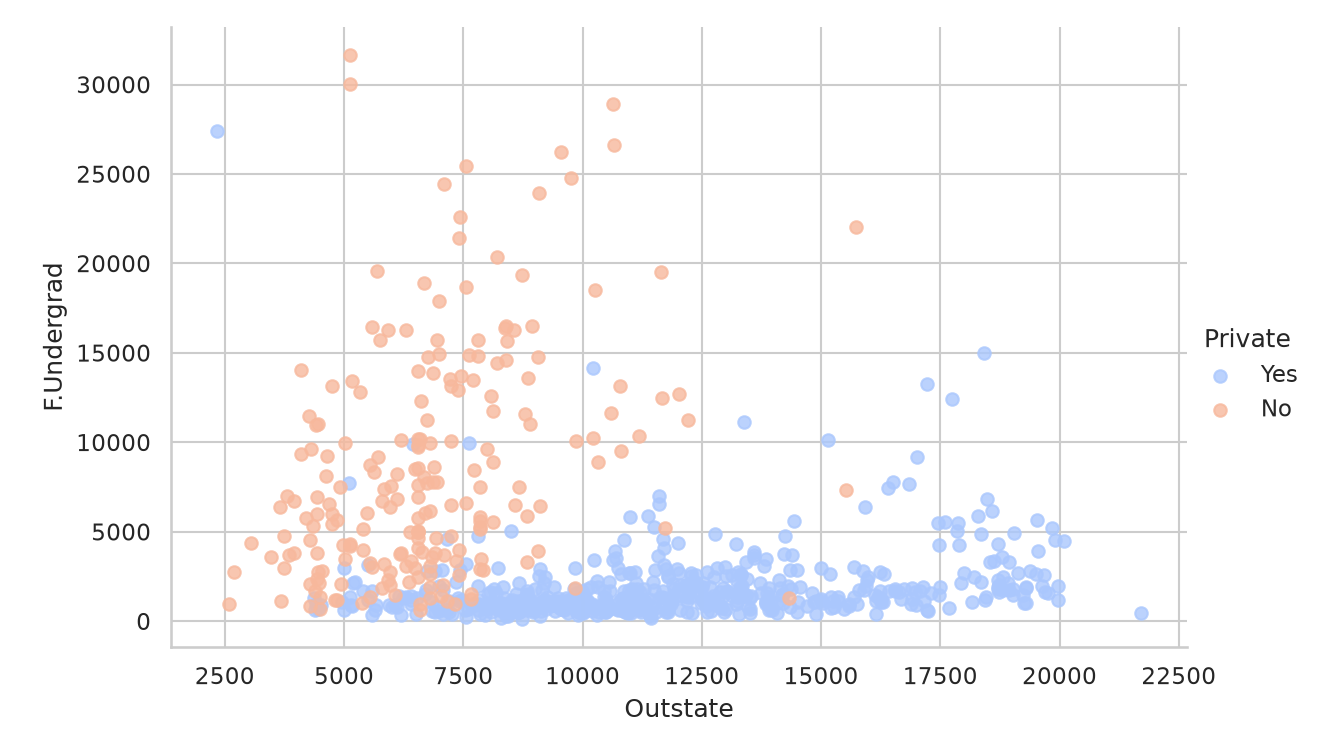
Three cells to fix
| Cell | Problem | Fix |
|---|---|---|
pd.read_csv('College_Data', index_col=0) | the file is not next to the notebook in Colab | read it from the repository's Datasets folder (below) |
df['Grad.Rate']['Cazenovia College'] = 100 | chained assignment; with pandas 3 it prints a ChainedAssignmentError warning and the value stays 118 | df.loc['Cazenovia College', 'Grad.Rate'] = 100 |
sns.lmplot('Room.Board','Grad.Rate', ..., size=6) and sns.FacetGrid(..., size=6) | current seaborn needs x= and y= by name and calls size height | sns.lmplot(x='Room.Board', y='Grad.Rate', data=df, hue='Private', palette='coolwarm', height=6, aspect=1, fit_reg=True) |
url = ("https://raw.githubusercontent.com/"
       "tirthajyoti/Machine-Learning-with-Python/"
       "master/Datasets/College_Data")
df = pd.read_csv(url, index_col=0)
df.loc['Cazenovia College', 'Grad.Rate'] = 100
Cazenovia College reports a graduation rate of 118, which is impossible, so the notebook sets it to 100.
Fit two clusters
from sklearn.cluster import KMeans

kmeans = KMeans(n_clusters=2, verbose=0, tol=1e-3, max_iter=300, n_init=20, random_state=0)
kmeans.fit(df.drop('Private', axis=1))
We added random_state=0 so the run is repeatable. n_init=20 runs the algorithm from 20 starts and keeps the best; tol and max_iter control when a run stops. We tried random_state from 0 to 9, and every run ends in the same two clusters with the same inertia: 669 colleges in one cluster and 108 in the other. With random_state=0, the 669 are cluster 0.
Four of the 17 centroid coordinates, from kmeans.cluster_centers_:
| Feature | Cluster 0 (669 colleges) | Cluster 1 (108 colleges) |
|---|---|---|
Apps | 1813.2 | 10363.1 |
F.Undergrad | 2188.5 | 13061.9 |
Outstate | 10395.7 | 10719.2 |
Expend | 8932.0 | 14170.5 |
Cluster 1 holds the big colleges: many applications, many students, high spending per student. Cluster 0 holds the small ones.
Compare the clusters with the labels
The notebook turns Private into a 0 or 1 column (1 for a private college) and compares it with kmeans.labels_:
from sklearn.metrics import confusion_matrix, classification_report

def converter(cluster):
    if cluster == 'Yes':
        return 1
    else:
        return 0

df['Cluster'] = df['Private'].apply(converter)
print(confusion_matrix(df['Cluster'], kmeans.labels_))
[[138 74]
[531 34]]Rows are the true label (0 public, 1 private) and columns the cluster. The "correct" cells hold 138 + 34, so the accuracy is 172 / 777 = 0.2214. That looks terrible, but it is a naming problem: k-means called the small colleges cluster 0, while the label calls private colleges 1. Most private colleges (531 of 565) are in cluster 0.
Swap the two cluster numbers with 1 - kmeans.labels_:
print(confusion_matrix(df['Cluster'], 1 - kmeans.labels_))
print(classification_report(df['Cluster'], 1 - kmeans.labels_))
[[ 74 138]
[ 34 531]]
precision recall f1-score support
0 0.69 0.35 0.46 212
1 0.79 0.94 0.86 565
accuracy 0.78 777
macro avg 0.74 0.64 0.66 777
weighted avg 0.76 0.78 0.75 777This is the matrix saved in the notebook, whose run happened to number the clusters the other way.
- Accuracy:
(74 + 531) / 777 = 605 / 777 = 0.7786. - Private colleges: precision
531 / (531 + 138) = 0.7937, recall531 / 565 = 0.9398. - Public colleges: precision
74 / (74 + 34) = 0.6852, recall74 / 212 = 0.3491.
k-means found size, not ownership: the "big" cluster of 108 colleges contains 74 public and 34 private colleges, and 138 public colleges are small enough to sit with the private ones. The features with the largest numbers (Expend, F.Undergrad, Outstate, Apps) dominate the distance.
A copy that is not a copy
Before its last cell the notebook writes df1 = df and then adds the Cluster column to df1. That line does not copy anything: df1 and df are the same DataFrame, so df now contains the true labels too. The last cell fits KMeans again on df.drop('Private', axis=1), which now includes Cluster, so the model is secretly given the answer. Use df1 = df.copy() when you need a real copy.
Common mistakes
- Treating the cluster numbers as meaningful. Cluster 0 in one run can be cluster 3 in another; read the centroids.
- Picking the k with the smallest inertia. Inertia always falls as k grows; look for the elbow.
- Trusting a single start. Use
n_init=10or more, and fixrandom_statewhen you need the same result again. - Clustering on an ID column.
CustomerIDis a row number, not a property of the customer. - Passing text columns to
KMeans. Encode them first, for example withLabelEncoder. - Scoring clusters against labels without first matching the cluster numbers to the labels.
- Writing
df1 = dfwhen you meandf1 = df.copy().
Project milestone: presentations and discussions
This week's milestone is Project Teams Presentations and Discussions. Each team presents its project and answers questions. Prepare:
- The problem your project solves and the dataset you use: rows, features and the target.
- How you cleaned and explored the data, with one or two plots.
- The models you built since week 3, and their scores on the same test split.
- The model you keep, and why.
- What is still missing, and your plan for it.
If your data has no labels, or you want to find groups in it, try k-means on it and show the elbow curve and the centroids of your clusters.
Key takeaways
- Clustering finds groups in data that has no labels.
- k-means repeats two steps: assign every point to its nearest centroid, then update every centroid to the mean of its points, until nothing changes.
- The WCSS (
inertia_) measures how tight the clusters are; neither step can increase it. - Choose k with the elbow method, not with the smallest inertia.
- The result depends on the start: use
n_initto try several starts. - The clusters are numbered arbitrarily; a person reads the centroids and names the segments.
Practice
About 30 minutes. Try each task before you read its answer at the end of the page.
Practice 1: a different start (about 10 minutes)
Use the same five customers as the worked example, with k = 2, but start the centroids at μ1 = #11 = (19, 14) and μ2 = #136 = (73, 88).
- Run the assign step and the update step until no customer changes cluster.
- Write down the final clusters, the final centroids and the final J.
- How many assign steps did you need, compared with the worked example?
Practice 2: which segment? (about 5 minutes)
The five customer segments of Part 3 have these centroids (rounded to one decimal):
| Cluster | Centroid (income, spending) |
|---|---|
| 0 | (55.3, 49.5) |
| 1 | (86.5, 82.1) |
| 2 | (88.2, 17.1) |
| 3 | (26.3, 20.9) |
| 4 | (25.7, 79.4) |
A new customer has an income of 100 and a spending score of 50. Compute the squared distance to every centroid. Which segment does the customer join? Is it a close call?
Practice 3: score the college clusters (about 5 minutes)
After swapping the cluster numbers, the colleges give this confusion matrix (rows: true label, columns: cluster):
| Cluster 0 | Cluster 1 | |
|---|---|---|
| Public (0) | 74 | 138 |
| Private (1) | 34 | 531 |
Compute the accuracy, and the precision and recall of the private class.
Practice 4: in Colab (about 10 minutes)
- Run notebook 1 up to the five segments on income and spending. Predict the segment of the customers
[[100, 50], [20, 90]]with one call tokmeans.predict. - Re-run the four-feature model with
n_init=10. Printkmeans.inertia_and the size of each cluster withnp.bincount(kmeans.labels_). - In notebook 2, fit the two-cluster model with
random_state=2instead of 0. Print the confusion matrix and the accuracy withaccuracy_scorefromsklearn.metrics.
Answers
Answer 1
Iteration 1, assign:
| Customer | d² to μ1 (19, 14) | d² to μ2 (73, 88) | Joins |
|---|---|---|---|
| #11 | 0 | 2916 + 5476 = 8392 | μ1 |
| #49 | 441 + 784 = 1225 | 1089 + 2116 = 3205 | μ1 |
| #62 | 729 + 1681 = 2410 | 729 + 1089 = 1818 | μ2 |
| #136 | 8392 | 0 | μ2 |
| #190 | 7056 + 5041 = 12097 | 900 + 9 = 909 | μ2 |
J after this step: 0 + 1225 + 1818 + 0 + 909 = 3952.
Iteration 1, update: μ1 = mean of #11 and #49 = (29.5, 28); μ2 = mean of #62, #136 and #190 = (74, 76).
These are exactly the centroids of iteration 3 in the worked example, so the rest is the same:
- Iteration 2, assign: #62 moves to μ1 (1001.25 against 1225); J = 2680.75.
- Iteration 2, update: μ1 = (35, 37), μ2 = (88, 86.5); J = 1734.5.
- Iteration 3, assign: nobody moves. Converged.
The final clusters are (#11, #49, #62) and (#136, #190), with J = 1734.5, the same as the worked example. This start needed 3 assign steps instead of 4, because it began closer to the answer. With only five points, every pair of starting customers ends in this same result; on bigger data, as Part 3 showed, different starts can end in different results.
Answer 2
| Cluster | Differences | Squared distance |
|---|---|---|
| 0 | 44.7, 0.5 | 1998.09 + 0.25 = 1998.34 |
| 1 | 13.5, -32.1 | 182.25 + 1030.41 = 1212.66 |
| 2 | 11.8, 32.9 | 139.24 + 1082.41 = 1221.65 |
| 3 | 73.7, 29.1 | 5431.69 + 846.81 = 6278.50 |
| 4 | 74.3, -29.4 | 5520.49 + 864.36 = 6384.85 |
The customer joins cluster 1 (high income, high spending), but only just: cluster 2 is 1221.65, less than 9 more. With the unrounded centroids the two values are 1213.43 and 1220.71, and kmeans.predict([[100, 50]]) also returns cluster 1. A customer on the border between two segments is a reminder that segments are a simplification.
Answer 3
- Accuracy:
(74 + 531) / 777 = 605 / 777 = 0.7786. - Precision of the private class:
531 / (531 + 138) = 531 / 669 = 0.7937. - Recall of the private class:
531 / (531 + 34) = 531 / 565 = 0.9398.
The model finds 94 percent of the private colleges, but 138 public colleges land in the same cluster.
Answer 4
kmeans.predict(np.array([[100, 50], [20, 90]]))returns[1 4]: the first customer joins the high income, high spending segment (as in Answer 2), and the second joins the low income, high spending segment.- With
n_init=10:kmeans.inertia_is about75399.6154(75399.62 rounded; the last digits of the printed value can differ from one machine to another), andnp.bincount(kmeans.labels_)is[23 39 79 23 36]. - With
random_state=2, the same two clusters come out with the other numbering:
[[ 74 138]
 [ 34 531]]
0.7786357786357786
The accuracy jumps from 0.2214 to 0.7786 only because the names of the two clusters changed. Nothing about the clustering itself changed: the inertia is the same in both runs.