

In the print dialog, choose "Save as PDF" as the destination.
Machine Learning, Week 6
Decision Trees and Random Forest
Classify a borrower by asking questions, then let many trees vote: the Lending Club loans.
Objectives
- ▸Explain how a decision tree classifies: a chain of threshold questions that ends in a leaf
- ▸Compute the Gini impurity of a node and the weighted Gini of a split by hand
- ▸Explain why a tree grown until every leaf is pure overfits
- ▸Explain a random forest: bootstrap samples, random features at each split, a vote
- ▸Train
DecisionTreeClassifierandRandomForestClassifieron the Lending Club data - ▸Spot when a high accuracy only reflects an unbalanced target, and apply it to your project
Week 6 of the plan
Where This Sits in the Course
- ▸One notebook: DecisionTrees_RandomForest_Classification, a tree and a forest on public lending data
- ▸Real-world scenario: Lending Club connects borrowers with investors; predict whether a borrower paid back the loan in full
- ▸Project milestone: Machine Learning Model Implementation, continued on your own data
Plan for the Two Hours
| Part | What we do | Time |
|---|---|---|
| 1 | The idea of a tree, and a tree grown by hand | 30 min |
| 2 | The Lending Club notebook: data and exploration | 15 min |
| 3 | One decision tree on the loans | 10 min |
| 4 | Random forest: by hand, then on the loans | 25 min |
| 5 | Mistakes, project, practice with answers, takeaways | 40 min |
Part 1
The Idea of a Decision Tree
Ask questions until the answer is clear
What Is a Decision Tree?
- Decision tree
- A classifier that asks a chain of yes or no questions, each comparing one feature with a threshold, such as
fico ≤ 677.
- ▸Yes sends the sample down the left branch, no down the right one
- ▸The next question waits at the end of each branch
- ▸A node with no question is a leaf: its class is the prediction
The Vocabulary, on the Loans
| Term | In the Lending Club data |
|---|---|
Features X | credit data, such as fico (credit score) and int.rate (interest rate) |
Label y | not.fully.paid: 1 did not pay back in full, 0 paid in full |
| Root node | the first question, asked of every borrower |
| Leaf | a node with no question: it predicts its majority class |
| Depth | the number of questions on the longest path to a leaf |
How Mixed Is a Node? Gini Impurity
The notebook trains with criterion='gini'
- ▸
p_0is the fraction of the node in class0(paid),p_1in class1(not paid)
Choosing a Question: the Weighted Gini
- ▸A question splits
nrows inton_Lon the left andn_Ron the right - ▸
G_L,G_Rare the Gini of each side; each side counts by its size - ▸Candidate thresholds are the midpoints between neighbouring values
By hand
Worked Example: Ten Real Borrowers
Rows of loan_data.csv, sorted by fico. y = 1: not paid in full. Four of ten did not pay.
| Borrower | fico | int.rate | y |
|---|---|---|---|
| B1 | 647 | 0.1482 | 1 |
| B2 | 662 | 0.1507 | 0 |
| B3 | 667 | 0.1299 | 1 |
| B4 | 672 | 0.1347 | 1 |
| B5 | 682 | 0.1103 | 0 |
| Borrower | fico | int.rate | y |
|---|---|---|---|
| B6 | 687 | 0.1387 | 0 |
| B7 | 692 | 0.1284 | 0 |
| B8 | 707 | 0.1091 | 1 |
| B9 | 727 | 0.1059 | 0 |
| B10 | 757 | 0.1189 | 0 |
Step 1: The Gini of the Root
All ten borrowers: 6 paid, 4 not paid
Step 2: Try the Question fico ≤ 677
677 is the midpoint between B4 (672) and B5 (682)
| Side | Borrowers | Not paid | Paid |
|---|---|---|---|
yes, ≤ 677 | B1 to B4 | 3 | 1 |
no, > 677 | B5 to B10 | 1 (B8) | 5 |
Step 3: The Gini of Each Side
Step 4: The Weighted Gini of the Split
Step 5: The Other Feature
The best question on int.rate is int.rate ≤ 0.12915
| Side | Borrowers | Not paid | Paid |
|---|---|---|---|
| yes, lower rates | B5, B7, B8, B9, B10 | 1 | 4 |
| no, higher rates | B1, B2, B3, B4, B6 | 3 | 2 |
Step 6: The Search Tries Every Threshold
Nine fico midpoints and nine int.rate midpoints: eighteen candidates
| fico threshold | Left: not paid, paid | Right: not paid, paid | Weighted Gini |
|---|---|---|---|
| 654.5 | 1, 0 | 3, 6 | 0.4000 |
| 669.5 | 2, 1 | 2, 5 | 0.4190 |
| 677 | 3, 1 | 1, 5 | 0.3167 |
| 684.5 | 3, 2 | 1, 4 | 0.4000 |
| 717 | 4, 4 | 0, 2 | 0.4000 |
Step 7: Grow the Left Child
B1 to B4: 3 not paid, 1 paid, G = 0.375
Step 8: Grow the Right Child
B5 to B10: 1 not paid (B8), 5 paid, G = 0.2778
The Tree We Built
fico <= 677 ?
|-- yes: int.rate <= 0.14945 ?
|        |-- yes: leaf [3 not paid, 0 paid] -> not paid
|        |-- no:  leaf [0 not paid, 1 paid] -> paid
|-- no:  int.rate <= 0.1097 ?
         |-- yes: leaf [1 not paid, 1 paid] -> paid
|-- no: leaf [0 not paid, 4 paid] -> paidPredict Two New Borrowers
Follow the questions from the root
- ▸A:
670 ≤ 677yes, then0.14 ≤ 0.14945yes, so the leaf says not paid
- ▸B:
700 ≤ 677no, then0.12 ≤ 0.1097no, so the leaf says paid
Try It: Grow the Tree Yourself
Part 2
The Lending Club Notebook
9578 real loans, 2007 to 2010
Open the Notebook in Colab
https://colab.research.google.com/github/
tirthajyoti/Machine-Learning-with-Python/blob/
master/Classification/
DecisionTrees_RandomForest_Classification.ipynbLoad and Inspect the Data
import pandas as pd

url = ("https://raw.githubusercontent.com/"
       "tirthajyoti/Machine-Learning-with-Python/"
       "master/Datasets/loan_data.csv")
df = pd.read_csv(url)
df.info()- ▸9578 rows, 14 columns, no missing values
- ▸
fico: credit score;int.rate: interest rate as a proportion - ▸
purpose: the loan purpose, as text - ▸Label
not.fully.paid:1if not paid back in full
The Count That Matters
print(df['not.fully.paid'].value_counts())| not.fully.paid | Borrowers | Share |
|---|---|---|
| 0, paid | 8045 | 84% |
| 1, not paid | 1533 | 16% |
Explore Before You Model
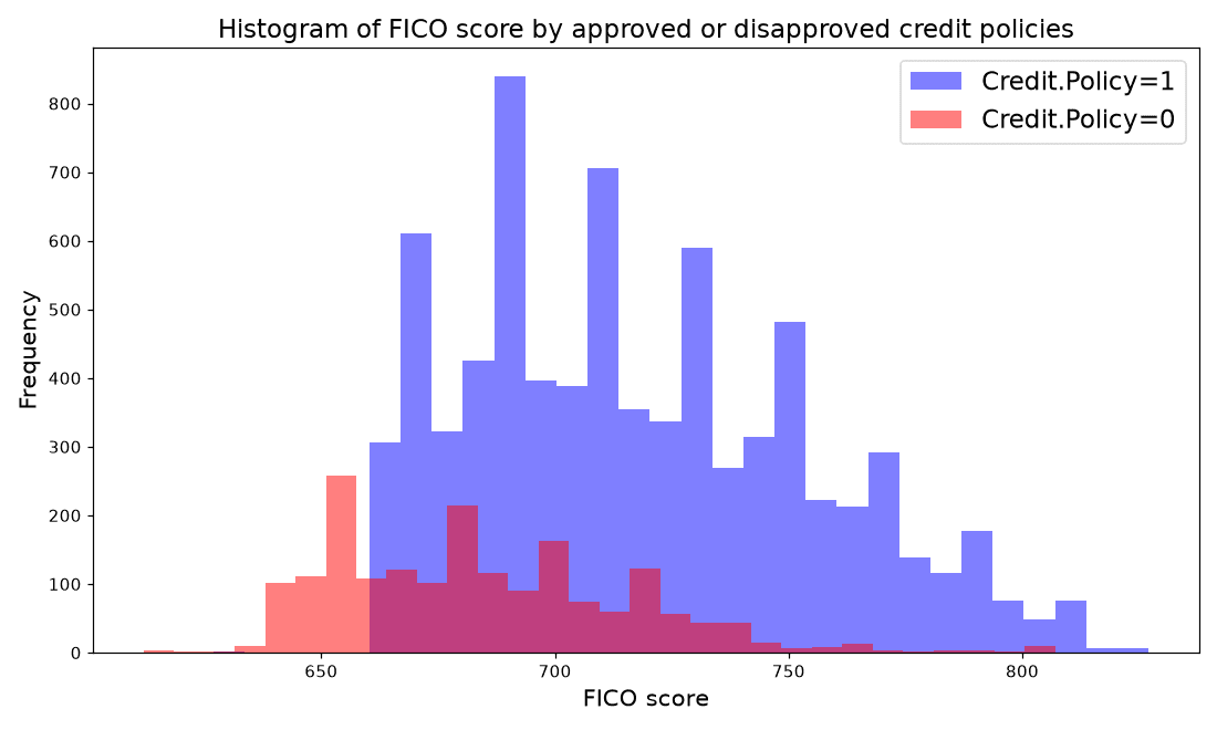
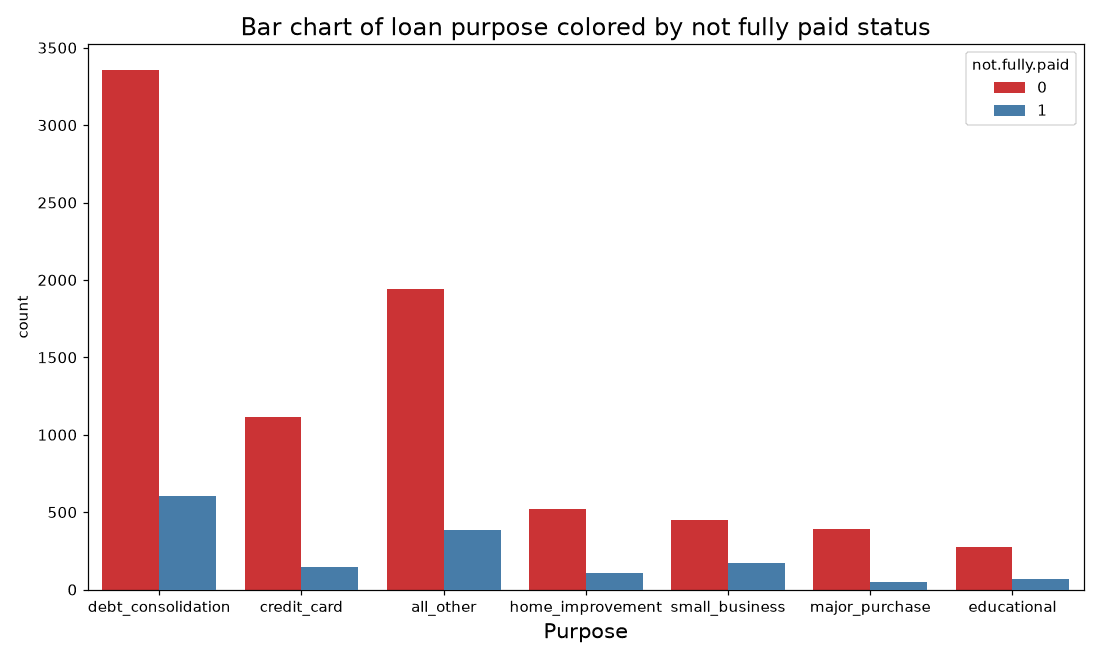
- ▸Below
fico 660: 487 borrowers fail the credit policy, only 2 pass. One threshold separates a group - ▸Not paid in full: 27.8% of
small_businessloans, 11.6% ofcredit_cardloans
Turn the Text Column into Numbers
df_final = pd.get_dummies(df, ['purpose'],
drop_first=True)- ▸Seven purposes become six 0 or 1 columns, such as
purpose_credit_card - ▸
drop_first=Truedropsall_other: all six at 0 means that purpose - ▸
df_finalhas 19 columns
Split into Training and Test Sets
X = df_final.drop('not.fully.paid', axis=1)
y = df_final['not.fully.paid']
X_train, X_test, y_train, y_test = train_test_split(
X, y, test_size=0.30, random_state=101)Part 3
One Decision Tree on the Loans
Let the tree grow until every leaf is pure
Fit the Tree and Predict
from sklearn.tree import DecisionTreeClassifier

dtree = DecisionTreeClassifier(criterion='gini', max_depth=None,
                               random_state=101)
dtree.fit(X_train, y_train)
predictions = dtree.predict(X_test)- ▸
criterion='gini': the impurity from Part 1 - ▸
max_depth=None: keep splitting until every leaf is pure - ▸
random_state=101: ties between equally good splits break the same way every run
The Tree's Confusion Matrix
A: accuracy. R_1, P_1: recall and precision of class 1
| Predicted 0 (paid) | Predicted 1 (not paid) | |
|---|---|---|
| Actual 0 | 1975 | 456 |
| Actual 1 | 336 | 107 |
The Tree Memorised Its Training Set
print(dtree.get_depth(), dtree.get_n_leaves())
print(dtree.score(X_train, y_train))| Measure | Value |
|---|---|
| Depth | 27 |
| Leaves | 1005 |
| Training accuracy | 1.0 |
Part 4
Random Forest
Many different trees, one vote
The Idea: Many Different Trees
- 1Bootstrap: each tree gets
nrows drawn at random with replacement from thentraining rows - 2Random features: at every split a tree searches only
mof thepfeatures,m = ⌊√p⌋ - 3Vote: every tree classifies the new sample; the majority class wins
By hand
Worked Example: One Bootstrap Sample
RandomForestClassifier(n_estimators=5, random_state=0) on the ten borrowers. With p = 2, every split searches m = 1 random feature
- ▸Tree 1 drew: B4, B3, B1, B1, B3, B7, B10, B8, B4, B10
- ▸Twice: B1, B3, B4, B10. Once: B7, B8
- ▸Never drawn: B2, B5, B6, B9, left out of this tree
Five Trees Vote on a New Borrower
New borrower: fico 710, int.rate 0.11
| Tree | Left out of its sample | Vote |
|---|---|---|
| 1 | B2, B5, B6, B9 | not paid |
| 2 | B3, B6, B7 | paid |
| 3 | B1, B3, B7, B10 | paid |
| 4 | B2, B3, B7, B8, B10 | paid |
| 5 | B1, B3, B5, B9 | not paid |
Try It: Watch the Forest Vote
Fit the Forest
from sklearn.ensemble import RandomForestClassifier

rfc = RandomForestClassifier(n_estimators=600, random_state=101)
rfc.fit(X_train, y_train)
rfc_pred = rfc.predict(X_test)
print(confusion_matrix(y_test, rfc_pred))
print(classification_report(y_test, rfc_pred))p = 18, each split searches m = 4 features: rfc.estimators_[0].max_features_ prints 4.The Forest's Confusion Matrix
A: accuracy on the 2874 test borrowers
| Predicted 0 (paid) | Predicted 1 (not paid) | |
|---|---|---|
| Actual 0 | 2420 | 11 |
| Actual 1 | 431 | 12 |
Do You Get Anything Strange?
A_0: accuracy of "paid" for everyone. R_1: recall of class 1
- ▸The forest flags only 23 borrowers and beats "paid for everyone" by one
- ▸No test borrower gets more than 375 of the 600 trees voting "not paid"
How Many Trees?
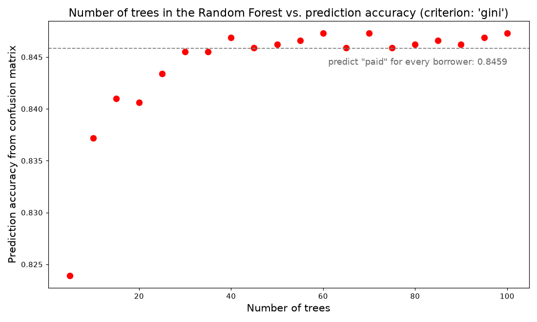
- ▸The notebook loops over 5 to 100 trees,
min_samples_split=10; we addrandom_state=101to each forest - ▸0.8239 with 5 trees, then 0.8455 to 0.8473 from 30 trees on
- ▸More trees steady the vote, but the curve settles at the level of "paid for everyone"
Before you practise
Common Mistakes
- ▸Reading
loan_data.csvin Colab from a folder that does not have it - ▸Forgetting
random_state, then comparing numbers from two different splits - ▸Trusting the perfect training score of a tree grown with
max_depth=None - ▸Judging a model by accuracy alone when one class is rare
- ▸Printing the report of
predictionswhen you meantrfc_pred - ▸Passing a text column such as
purposewithout dummy variables
Your team project
Project Milestone: Model Implementation
- 1Take last week's features and target; turn text columns into dummies
- 2Split with a fixed
random_state - 3Fit
DecisionTreeClassifier: compare its training and test scores - 4Fit
RandomForestClassifier: report the confusion matrix andclassification_report - 5Compare tree, forest and KNN on the same test set, using the recall of every class
Part 5
Practice: Your Turn
About 30 minutes, answers follow each task
About 10 minutes
Practice 1: Choose the First Question
Eight other real borrowers, y = 1: not paid
| Borrower | fico | int.rate | y |
|---|---|---|---|
| P1 | 647 | 0.1482 | 1 |
| P2 | 667 | 0.1343 | 0 |
| P3 | 677 | 0.1734 | 1 |
| P4 | 682 | 0.1197 | 0 |
| Borrower | fico | int.rate | y |
|---|---|---|---|
| P5 | 692 | 0.1287 | 0 |
| P6 | 697 | 0.1316 | 1 |
| P7 | 742 | 0.1114 | 0 |
| P8 | 747 | 0.0751 | 0 |
- ▸Compute the Gini of the root
- ▸Compute
G_wforfico ≤ 679.5and forint.rate ≤ 0.13015 - ▸Which question wins, and by how much does the Gini fall?
Answers
Practice 1: Answer
| Question | Weighted Gini |
|---|---|
fico ≤ 679.5 | G_w = 0.375 × 0.4444 + 0.625 × 0.32 ≈ 0.3667 |
int.rate ≤ 0.13015 | G_w = 0.5 × 0 + 0.5 × 0.375 = 0.1875 |
About 5 minutes
Practice 2: Read the Forest's Matrix
The 600-tree forest: [[2420, 11], [431, 12]]
About 5 minutes
Practice 3: Entropy of the First Split
The notebook also trains with criterion='entropy'
About 10 minutes
Practice 4: In Colab, on the Loans
- 1After the split with
random_state=101, fitDecisionTreeClassifier(max_depth=5, random_state=101) - 2Print its confusion matrix, its test and training accuracy; compare with
max_depth=None - 3Rerun the loop over the number of trees with
max_depth=5andrandom_state=101in each forest
| Tree | Confusion matrix | Test | Training |
|---|---|---|---|
max_depth=5 | [[2396, 35], [431, 12]] | 0.8379 | 0.845 |
max_depth=None | [[1975, 456], [336, 107]] | 0.724 | 1.0 |
Key Takeaways
- 1A tree classifies by a chain of threshold questions; a leaf predicts its majority class
- 2Each question is the one with the lowest weighted Gini over every feature and threshold
- 3A tree grown until every leaf is pure memorises its training set
- 4A random forest votes over trees grown on bootstrap samples with random features
- 5When one class is rare, read its recall, not only the accuracy
Open this lesson
Mahmoud Abas|Decision Trees and Random Forest