Mahmoud Abas, Full-Stack Software Engineer & AI

Machine Learning, Week 1

Advanced Pandas and Reading Data from Many Sources

Load data from CSV, text, Excel, HTML and JSON into a DataFrame, then filter, group, clean, join and reshape it.

Objectives

Read CSV and text files with the right sep, header, names, skiprows, skipfooter and nrows
Read Excel sheets, HTML tables and JSON files into a DataFrame
Select rows with loc and a boolean mask, and summarise columns with describe
Use groupby and pivot_table to aggregate, and apply to create new columns
Find and fix missing values with isnull, fillna and dropna
Combine tables with concat, merge and join

Week 1 of the plan

Where This Sits in the Course

Two notebooks: Advanced Pandas Operations and How to read data from different text based (and non-text based) sources
Data: a superstore file of 9994 orders, and small house-price files in many formats
Project milestone this week: form a team of 3 with a project idea, or a team of 2 with a research paper

Plan for the Two Hours

Part	What we do	Time
1	Reading data from many sources	35 min
2	Selecting, filtering and grouping	25 min
3	Missing values, joins and reshaping	25 min
4	Common mistakes and the project milestone	5 min
5	Practice with answers, then takeaways	30 min

Part 1

Reading Data from Many Sources

One function per format, one DataFrame at the end

One Function per Source

Source	pandas function	Returns
CSV, zipped CSV	`pd.read_csv`	a DataFrame
Other delimited text	`pd.read_table`	a DataFrame
Excel workbook	`pd.read_excel`	a DataFrame, or a dict of them
Tables in a web page	`pd.read_html`	a list of DataFrames
JSON file	`pd.read_json`	a DataFrame

Read the Files from the Repository

python

base = ("https://raw.githubusercontent.com/tirthajyoti/"
        "Machine-Learning-with-Python/master/Pandas%20and%20Numpy/"
        "Read_data_various_sources/")
df1 = pd.read_csv(base + "CSV_EX_1.csv")
df1.shape      # (5, 4)

A Clean CSV

CSV_EX_1.csv, five houses

text

Bedroom, Sq. foot, Locality, Price ($)
2, 1500, Good, 300000
3, 1300, Fair, 240000
3, 1900, Very good, 450000
3, 1850, Bad, 280000
2, 1640, Good, 310000

The raw file

python

df1 = pd.read_csv("CSV_EX_1.csv")
df1.shape      # (5, 4)

Line 1 becomes the column names
Each other line becomes one row
Numbers become int64, words stay text

Worked Example: A File with No Header

CSV_EX_2.csv holds the same five houses, without the header line

text

   2   1500        Good   300000
0  3   1300        Fair   240000
1  3   1900   Very good   450000
2  3   1850         Bad   280000
3  2   1640        Good   310000

The Fix: header=None and names

python

df2 = pd.read_csv("CSV_EX_2.csv",
    header=None,
    names=['Bedroom', 'Sq.ft',
           'Locality', 'Price($)'])

text

   Bedroom  Sq.ft    Locality  Price($)
0        2   1500        Good    300000
1        3   1300        Fair    240000
2        3   1900   Very good    450000
3        3   1850         Bad    280000
4        2   1640        Good    310000

Worked Example: Semicolons Instead of Commas

CSV_EX_3.csv: Bedroom; Sq. foot; Locality; Price ($)

df3.shape is (5, 1): no comma, so each line stays one text value
The fix is pd.read_csv("CSV_EX_3.csv", sep=';'), which gives (5, 4)

Worked Example: Extra Lines at the Top and Bottom

CSV_EX_skipfooter.csv

text

Filetype: CSV,,,
,Info about some houses,,
Bedroom, Sq. foot, Locality, Price ($)
2,1500, Good,300000
...
2,1640, Good,310000
, This is the end of file,,

(8, 4), columns Filetype: CSV, Unnamed: 1, Unnamed: 2, Unnamed: 3
The fix: skiprows=2, skipfooter=1, engine='python' gives the clean (5, 4)

Big Files: nrows and Reading in Chunks

python

rows_in_a_chunk = 10
num_chunks = 5
colnames = pd.read_csv("Boston_housing.csv", nrows=2).columns
list_of_dataframe = []
for i in range(0, num_chunks*rows_in_a_chunk, rows_in_a_chunk):
    df = pd.read_csv("Boston_housing.csv", header=0, skiprows=i,
                     nrows=rows_in_a_chunk, names=colnames)
    list_of_dataframe.append(df)

nrows=2 reads only the first 2 rows
Each pass skips i lines and reads the next 10
5 chunks, each of shape (10, 14)
Stacked together they equal the first 50 rows of the file (506 in total)

Worked Example: Blank Lines

CSV_EX_blankline.csv has two empty lines between the houses

Option	Shape	What you see
default (`True`)	(5, 4)	blank lines are skipped
`skip_blank_lines=False`	(7, 4)	two rows of NaN, and `2` becomes `2.0`

Try It: The read_csv Explorer

Zipped CSV Files

pd.read_csv("CSV_EX_1.zip") sees the .zip extension and unzips on the fly
No extra argument is needed: compression defaults to 'infer'
The result equals the plain CSV_EX_1.csv read

Excel: One Sheet or Every Sheet

python

pd.read_excel("Housing_data.xlsx", sheet_name='Data_Tab_1')

Sheet	Shape
`Data_Tab_1`	(9, 14)
`Data_Tab_2`	(4, 14)
`Data_Tab_3`	(16, 14)

read_table Expects Tabs

python

pd.read_table("Table_tab_separated.txt")   # (5, 4)
pd.read_table("Table_EX_1.txt")             # (5, 1)
pd.read_table("Table_EX_1.txt", sep=',')    # (5, 4)

read_table is read_csv with a tab as the default sep
Table_tab_separated.txt uses tabs: a clean (5, 4)
Table_EX_1.txt uses commas: one column, (5, 1), until you pass sep=','

Tables from a Web Page

pd.read_html(url, header=0) returns a list, one DataFrame per HTML table

Rank	NOC	Gold	Total
1	United States	46	121
2	Great Britain	27	67
3	China	26	70
4	Russia‡	19	56
5	Germany	17	42

Reading JSON

text

[
  {"Bedroom": 2, "Sq. foot": 1500,
   "Locality": "Good", "Price ($)": 300000},
  ...
]

houses.json: the five houses as JSON

python

dj = pd.read_json('houses.json')
dj[dj['Locality'] == 'Good']   # rows 0 and 4

read_json turns a list of records into rows: the same (5, 4) table
The column names come with no stray spaces
Filtering works as on any DataFrame: rows 0 and 4 are Good

Stata and PDF Files

pd.read_stata("rscfp2016.dta") reads a Stata data file the same way
read_pdf from the separate tabula-py package extracts tables from PDF pages
It returns a list of DataFrames and runs Java behind the scenes
PDF headers are hard to read, so the notebook passes names through pandas_options

Part 2

Selecting, Filtering and Grouping

The Advanced Pandas Operations notebook, on the superstore orders

Open the Notebook in Colab

text

https://colab.research.google.com/github/
tirthajyoti/Machine-Learning-with-Python/blob/master/
Pandas%20and%20Numpy/Advanced%20Pandas%20Operations.ipynb

Join the three lines into one address, or use the Open in Colab link on the lesson page.

The notebook reads Sample - Superstore.xls from its own folder, which Colab does not have
The next slide reads the same file from the repository instead

Load the Superstore Orders

python

url = ("https://raw.githubusercontent.com/tirthajyoti/"
       "Machine-Learning-with-Python/master/"
       "Pandas%20and%20Numpy/Sample%20-%20Superstore.xls")
df = pd.read_excel(url)
df.shape                          # (9994, 21)
df.drop('Row ID', axis=1, inplace=True)
df.shape                          # (9994, 20)

One row per order line: dates, ship mode, customer, place, product, Sales, Quantity, Discount, Profit
The workbook has 4 sheets: Orders, Returns, People, Missing

Pick Rows and Columns with loc

loc takes a list of index labels and a list of column names

python

df.loc[[i for i in range(5, 10)],
       ['Customer ID', 'City', 'Postal Code', 'Sales']]

Row	Customer ID	City	Sales
5	BH-11710	Los Angeles	48.860
6	BH-11710	Los Angeles	7.280
7	BH-11710	Los Angeles	907.152
8	BH-11710	Los Angeles	18.504
9	BH-11710	Los Angeles	114.900

Worked Example: describe on Records 100 to 199

python

df_subset = df.loc[[i for i in
    range(100, 200)], ['Sales', 'Profit']]
df_subset.describe()

Statistic	Sales	Profit
mean	262.957	0.348
std	858.984	170.745
min	1.788	-1359.992
50% (median)	66.960	9.654
max	8159.952	585.552

The Boxplot of the Same 100 Records

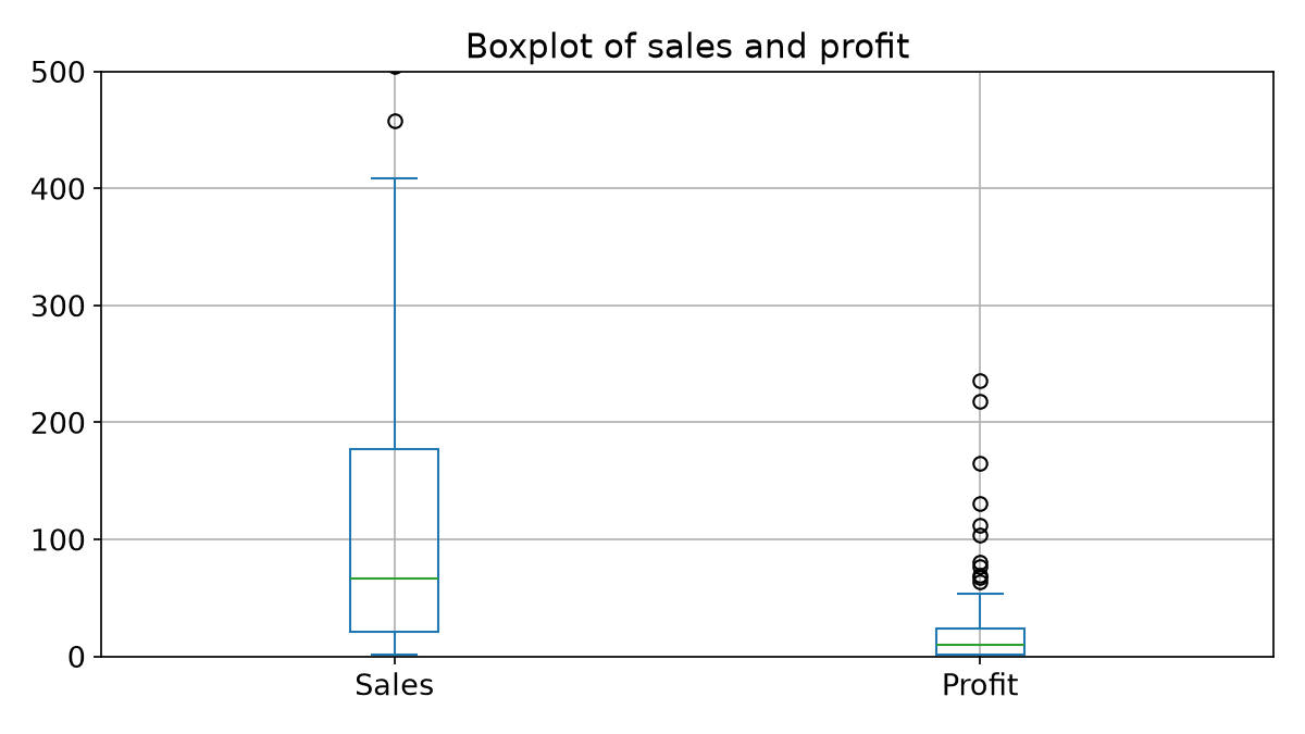
Boxplot of Sales and Profit for records 100 to 199, y axis cut at 0 and 500

df_subset.plot.box() draws one box per column
The box spans the middle half: Sales 21.3 to 177.1
plt.ylim(0, 500) zooms in: 12 sales and 1 profit above 500, and 20 negative profits, are off the chart

python

df_subset.plot.box()
plt.ylim(0, 500)
plt.grid(True)

Worked Example: A Boolean Mask

df_subset = df.loc[[i for i in range(10)], ['Ship Mode', 'State', 'Sales']]

text

        Ship Mode       State     Sales
0    Second Class    Kentucky  261.9600
1    Second Class    Kentucky  731.9400
2    Second Class  California   14.6200
3  Standard Class     Florida  957.5775
4  Standard Class     Florida   22.3680
5  Standard Class  California   48.8600
6  Standard Class  California    7.2800
7  Standard Class  California  907.1520
8  Standard Class  California   18.5040
9  Standard Class  California  114.9000

Combine Conditions with & and |

python

df_subset[(df_subset['State'] != 'California') & (df_subset['Sales'] > 100)]

Rows 0, 1, 3: rows 7 and 9 are in California
& means both, | means either, and each condition needs its own parentheses

groupby: Split, Apply, Combine

Split

rows by State

Apply

mean of each group

Combine

one row per State

python

byState = df_subset.groupby('State')
byState.mean(numeric_only=True)

Worked Example: Mean Sales per State

m_F = 957.5775 + 22.3682 = 489.97275

m_K = 261.96 + 731.942 = 496.95

groupby in Current pandas

Notebook code	Today	Write instead
`byState.mean()`	`TypeError`: text columns cannot be averaged	`byState.mean(numeric_only=True)`
`byState.sum()`	glues the Ship Mode text together	`byState.sum(numeric_only=True)`
`byState['Sales'].mean()`	works	the same, as a Series

Try It: DataFrame Operations, Step by Step

Part 3

Missing Values, Joins and Reshaping

The Missing sheet and small slices of the orders

Find the Missing Values

python

df_missing = pd.read_excel(url, sheet_name='Missing')
for c in df_missing.columns:
    miss = df_missing[c].isnull().sum()
    if miss > 0:
        print('{} has {} missing value(s)'.format(c, miss))
    else:
        print('{} has NO missing value!'.format(c))

text

Customer has 1 missing value(s)
Product has 2 missing value(s)
Sales has 1 missing value(s)
Quantity has 1 missing value(s)
Discount has NO missing value!
Profit has 1 missing value(s)

11 rows, 6 columns

Worked Example: Fill the Missing Sale

Sales rows 2 to 4 are 8.560, NaN, 22.720; the other 10 values add up to 3015.52

ffill() copies the value above: 8.56
bfill() copies the value below: 22.72

μ = 3015.5210 = 301.552

Worked Example: dropna

Call	What survives
`dropna(axis=0)`	?
`dropna(axis=1)`	?
`dropna(axis=1, thresh=10)`	?

axis=0: the 6 rows with no gap (1, 2, 4, 6, 9, 10)
axis=1: only Discount, the one full column
thresh=10: columns with at least 10 values, so only Product is dropped

Spotting Outliers with a Boxplot

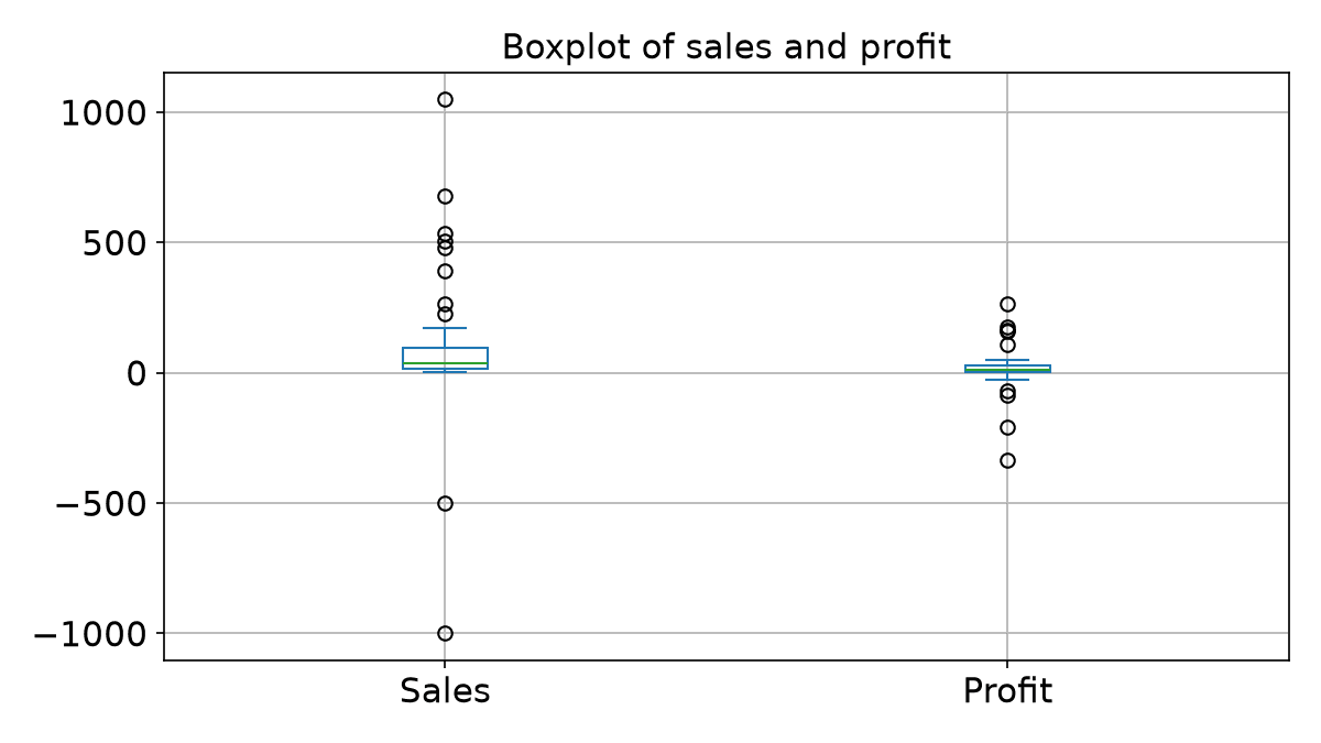
Boxplot of Sales and Profit for 50 sampled orders, with two planted negative sales at -1000 and -500

50 random orders, with two wrong sales planted: -1000 and -500
Sales can never be negative: the two points far below the box are the errors

Worked Example: concat

Three tables of 2 orders each, columns Customer ID, State, Sales, Profit, rows 0 to 5

axis=0 stacks rows: (6, 4)
axis=1 puts the tables side by side, matched on the index: (6, 12)
No row label is shared, so axis=1 leaves 48 of the 72 cells NaN

Worked Example: merge on a Key

df_1 and df_2: rows 0 to 3, keys CG-12520 twice, DV-13045, SO-20335

python

pd.merge(df_1, df_2, on='Customer ID', how='inner')

2 × 2 + 1 + 1 = 6

Inner, Left, Right, Outer

df_1 with df_3 (rows 2 to 5: DV-13045, SO-20335 twice, BH-11710)

how	Keeps	Rows
`inner`	keys in both tables	3
`left`	every df_1 row	5
`right`	every df_3 row	4
`outer`	every key, sorted	6

pivot_table: Averages per Region

python

df.pivot_table(values=['Sales', 'Quantity', 'Profit'], index=['Region'], aggfunc='mean')

Region	Profit	Quantity	Sales
Central	17.09	3.78	215.77
East	32.14	3.73	238.34
South	28.86	3.83	241.80
West	33.85	3.83	226.49

value_counts: The Quick Count

python

df['Ship Mode'].value_counts()

Ship Mode	Orders
Standard Class	5968
Second Class	1945
First Class	1538
Same Day	543

sort_values: Order the Rows

python

df_subset.sort_values(by='Sales')
df_subset.sort_values(by=['State', 'Sales'])

By Sales: row 6 (7.28) comes first and row 3 (957.5775) last
Each row keeps its index label
By ['State', 'Sales']: State first, then Sales breaks ties
So the six California rows lead, from 7.28 to 907.152

Worked Example: apply a Function

categorize_sales: Low below 50, Medium below 200, High otherwise

python

def categorize_sales(price):
    if price < 50:
        return "Low"
    elif price < 200:
        return "Medium"
    else:
        return "High"

df['Sales'].apply(categorize_sales)

High, Low, Medium
On all 9994 orders: Low 4849, High 2579, Medium 2566

Part 4

Common Mistakes and the Project Milestone

Five minutes before the practice

Before you practise

Common Mistakes

A single column after reading: the sep does not match the file
Losing the first row: the file has no header, so use header=None
Reading a local file name in Colab: use the repository address
Forgetting the parentheses around each condition joined by & or |
Old notebook calls: fillna(method=), mean() on text columns, chained assignment
Merging on a key that repeats and not checking the row count

Your team project

Project Milestone: Your Team

Form a team of 3 with a project idea, or a team of 2 with a research paper
Write down the question your project answers, or the paper you will study
Find the dataset and load it with the reader that fits its format
Check shape, the column names and isnull().sum() before anything else

Part 5

Practice: Your Turn

About 30 minutes, answers follow each task

About 5 minutes

Practice 1: A Messy Export

text

Exported by the lab system
Section 3
ID;Name;Quiz;Lab
101;A1;7;9
102;B2;5;8
103;C3;9;10
104;D4;6;7
End of export

p1_scores.txt

python

pd.read_csv('p1_scores.txt', sep=';', skiprows=2,
            skipfooter=1, engine='python')

About 8 minutes

Practice 2: Mask, groupby, apply

text

  Region       Ship Mode  Sales
0   East     First Class  120.0
1   West  Standard Class   45.5
2   East  Standard Class  310.0
3  South    Second Class   80.0
4   West     First Class  220.0
5  South  Standard Class   15.0
6   East    Second Class   95.0
7   West  Standard Class   60.5

Rows with Sales above 100 and Region not West
Sum and mean of Sales per Region
categorize_sales counts

Rows 0 and 2
Sums: East 525.0, South 95.0, West 326.0
Means: East 175.0, South 47.5, West 108.666667
Medium 4, Low 2, High 2

About 5 minutes

Practice 3: Missing Values

Qty = 4, NaN, 6, NaN, 10 and Price = 2.5, 3.0, NaN, 4.0, 5.5 and Item = pen, ink, None, pad, tape

ffill() and bfill() of Qty
Qty filled with its mean
Which rows survive dropna(axis=0)? Which columns survive dropna(axis=1, thresh=4)?

ffill: 4, 4, 6, 6, 10; bfill: 4, 6, 6, 10, 10
Mean 6.666667, so Qty becomes 4, 6.666667, 6, 6.666667, 10
Rows 0 and 4; columns Price and Item (Qty has only 3 values)

About 5 minutes

Practice 4: Count the Merge Rows

left: Key = K1, K2, K2, K3 with A = 1, 2, 3, 4. right: Key = K2, K3, K3, K4 with B = 10, 20, 30, 40

how	Rows	Why
`inner`	4	K2: 2 × 1, K3: 1 × 2
`left`	5	the 4 inner rows + K1 with NaN
`right`	5	the 4 inner rows + K4 with NaN
`outer`	6	the 4 inner rows + K1 + K4

About 7 minutes

Practice 5: In Colab, on the Superstore

How many orders come from Texas?
Total Sales and Profit per Category with groupby
How many orders lost money (Profit below 0)?
Total Profit per Region with pivot_table: which region is lowest?

Answers

Practice 5: Answers

Question	Answer
Texas orders	985
Sales per Category	Furniture 741999.80, Office Supplies 719047.03, Technology 836154.03
Profit per Category	Furniture 18451.27, Office Supplies 122490.80, Technology 145454.95
Orders with a loss	1871
Lowest Profit region	Central, 39706.36

Key Takeaways

One reader per format: read_csv, read_table, read_excel, read_html, read_json
Check the shape and column names right after reading: they reveal a wrong sep or header
Filter with a boolean mask, summarise with groupby and pivot_table
Find gaps with isnull, then decide: fill or drop
Join tables with concat, merge or join, and count the rows after

Open this lesson

Mahmoud AbasAdvanced Pandas and Reading Data from Many Sources