Mahmoud Abas, Full-Stack Software Engineer & AI

Machine Learning, Week 7

Naive Bayes Classification

Turn word counts into probabilities with Bayes' theorem, then build a spam filter and a wine classifier with scikit-learn.

Objectives

State Bayes' theorem and name its parts: prior, likelihood, evidence, posterior
Compute the probability of spam given a word from real counts
Explain the naive assumption and score an e-mail word by word, by hand
Explain why a count of 0 breaks the model and how Laplace smoothing fixes it
Build and evaluate a MultinomialNB spam filter with CountVectorizer
Train GaussianNB on numeric features: the wine data

Week 7 of the plan

Where This Sits in the Course

Two notebooks: E-Mail Classification (1000 labelled e-mails) and Naive_Bayes_Classification (178 wines)
Real-world scenario: spam e-mail detection, spam or legitimate (ham) from the words
Project milestone this week: Machine Learning Model Implementation

Plan for the Two Hours

Part	What we do	Time
1	Bayes' theorem, one word by hand	20 min
2	Naive Bayes by hand, and smoothing	30 min
3	Notebook 1: the spam filter	20 min
4	Notebook 2: Gaussian Naive Bayes on wine	20 min
5	Practice with answers, takeaways	30 min

Part 1

Bayes' Theorem

The Theorem and Its Four Parts

A conditional probability P(A | B): the probability of A, given that B is true. For a class c and evidence x:

P(c | x) = P(x | c) · P(c)P(x)

Part	Symbol	Meaning
Prior	`P(c)`	how common the class is, before looking
Likelihood	`P(x \| c)`	how common the evidence is inside the class
Evidence	`P(x)`	how common the evidence is overall
Posterior	`P(c \| x)`	the class probability after the evidence

By hand

Worked Example: Spam, Given the Word Money

999 e-mails. S spam, H ham, m: the e-mail contains money

Class	E-mails	Containing money
Spam `S`	500	79
Ham `H`	499	25
All	999	104

Step 1: The Prior and the Likelihood

P(S) = 500999 = 0.5005

P(m | S) = 79500 = 0.158

Step 2: The Evidence

P(m) = 79 + 25999 = 104999 = 0.1041

Step 3: The Posterior

P(S | m) = 0.158 × 0.50050.1041 = 0.7596

Part 2

Naive Bayes by Hand

The Naive Assumption

An e-mail has many words x_1, ..., x_n

P(x₁, x₂, ..., x_n | c) = P(x₁ | c) × P(x₂ | c) × ... × P(x_n | c)

The exact combination of words almost never repeats, so it cannot be counted
Naive Bayes assumes words are independent given the class
Then the likelihood is a product of one-word likelihoods
Real words are not independent, yet the method works surprisingly well

The Classification Rule

s(c) = P(c) × P(x₁ | c) × ... × P(x_n | c)

Compute the score s(c) for every class c
Predict the class with the largest score
Normalize: divide each score by the sum of all scores. That is predict_proba

Counting Words: MultinomialNB

P(w | c) = n_wc + αN_c + α V

Symbol	Meaning
`n_wc`	count of word `w` in the training e-mails of class `c`
`N_c`	total count of all vocabulary words in class `c`
`V`	number of words in the vocabulary
`α`	smoothing, `alpha=1.0` by default in `MultinomialNB()`

By hand

Worked Example: A Four-Word Spam Filter

Real counts in the 999 e-mails. Priors P(H) = 0.4995, P(S) = 0.5005, V = 4, α = 1

Word	Count in ham	Count in spam
`money`	38	155
`online`	7	94
`meeting`	153	1
`meds`	0	30
Total `N_c`	198	280

Step 1: Which Words Does the Filter See?

Vocabulary: money, online, meeting, meds

Step 2: The Word Probabilities

o = online, d = meds. Denominators: 198 + 4 = 202 for ham, 280 + 4 = 284 for spam

P(o | H) = 7 + 1202 = 0.0396

P(d | H) = 0 + 1202 = 0.00495

P(o | S) = 94 + 1284 = 0.3345

P(d | S) = 30 + 1284 = 0.1092

Step 3: The Two Scores

s(c) = P(c) times the word probabilities

s(H) = 0.4995 × 0.0396 × 0.00495 = 0.0000979

s(S) = 0.5005 × 0.3345 × 0.1092 = 0.0183

Step 4: Normalize

e = the e-mail

P(S | e) = 0.01830.0183 + 0.0000979 = 0.9947

P(H | e) = 1 - 0.9947 = 0.0053

Try It: The Spam Filter, Word by Word

The Zero-Count Problem

New e-mail e: Money for the meeting? The meeting is about meds. Counts: m = money 1, g = meeting 2, d = meds 1

P(d | H) = 0198 = 0

s(H) = 0.4995 × 0.1919 × 0.7727² × 0 = 0 ⇒ P(S | e) = 1

Laplace Smoothing Fixes It

α = 1: every count gets one extra, so no probability is ever 0

s(H) = 0.4995 × 0.1931 × 0.7624² × 0.00495 = 0.0002775

s(S) = 0.5005 × 0.5493 × 0.00704² × 0.1092 = 0.000001488

P(H | e) = 0.00027750.0002775 + 0.000001488 = 0.9947

Part 3

Notebook 1: The Spam Filter

Open the Notebook in Colab

text

https://colab.research.google.com/github/
jeffprosise/Machine-Learning/blob/master/
E-Mail%20Classification.ipynb

Join the three lines into one address, or click "Open in Colab" on the lesson page.

python

url = ("https://raw.githubusercontent.com/"
       "jeffprosise/Machine-Learning/master/Data/ham-spam.csv")
df = pd.read_csv(url)

The notebook reads Data/ham-spam.csv, which is not next to it in Colab. Read it from the repository.

Load the Data, Remove the Duplicate

python

df.info()
df.groupby('IsSpam').describe()
df = df.drop_duplicates()
df.groupby('IsSpam').describe()

1000 rows: IsSpam (0 ham, 1 spam) and Text
Text is already lower-case, no punctuation, nothing missing
500 ham rows but only 499 unique: one ham e-mail twice
After drop_duplicates(): 999 rows, 499 ham, 500 spam

Text to Counts: CountVectorizer

python

from sklearn.feature_extraction.text import CountVectorizer

vectorizer = CountVectorizer(
    ngram_range=(1, 2), stop_words='english')
x = vectorizer.fit_transform(df['Text'])
y = df['IsSpam']

One row per e-mail, one column per vocabulary entry, cells are counts
ngram_range=(1, 2): single words and pairs such as order online
stop_words='english': drops the, for, you...
x.shape is (999, 100687): 100687 columns

Worked Example: What the Vectorizer Keeps

python

text = vectorizer.transform(['Why pay MORE for * expensive meds when you can ...123... order them online and save $$$?'])
print(vectorizer.inverse_transform(text))

text

[array(['expensive', 'meds', 'online', 'order', 'order online', 'pay',
       'save'], dtype='<U401')]

Split and Train

python

from sklearn.model_selection import train_test_split
x_train, x_test, y_train, y_test = train_test_split(
    x, y, test_size=0.2, random_state=0)

from sklearn.naive_bayes import MultinomialNB
model = MultinomialNB()
model.fit(x_train, y_train)

799 e-mails to train, 200 to test (102 ham, 98 spam)
fit only counts: the priors and a smoothed P(w | c) for each of the 100687 columns

The Confusion Matrix

101 of 102 ham e-mails kept, 95 of 98 spam e-mails caught

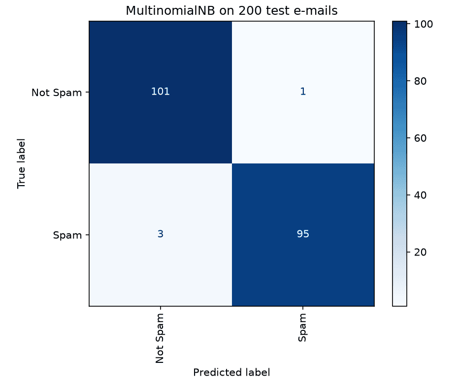
Confusion matrix of the spam filter on 200 test e-mails: 101 and 1 in the Not Spam row, 3 and 95 in the Spam row

python

from sklearn.metrics import ConfusionMatrixDisplay

ConfusionMatrixDisplay.from_estimator(
    model, x_test, y_test,
    display_labels=['Not Spam', 'Spam'],
    cmap='Blues', xticks_rotation='vertical')

Worked Example: Score the Spam Filter

A accuracy, P precision and R recall of spam

A = 101 + 95200 = 0.98

P = 9595 + 1 = 0.9896, R = 9595 + 3 = 0.9694

Classify New E-mails

python

message = vectorizer.transform(['Can you attend a code review on Tuesday? Need to make sure the logic is rock solid.'])
model.predict(message)[0]
model.predict_proba(message)[0][0]

message = vectorizer.transform(['Why pay more for expensive meds when you can order them online and save $$$?'])
model.predict(message)[0]
model.predict_proba(message)[0][1]

E-mail	predict	probability shown
code review	`0` (ham)	`P(H) = 0.99992`
expensive meds	`1` (spam)	`P(S) = 0.99979`

Part 4

Notebook 2: Gaussian Naive Bayes on Wine

The Wine Data

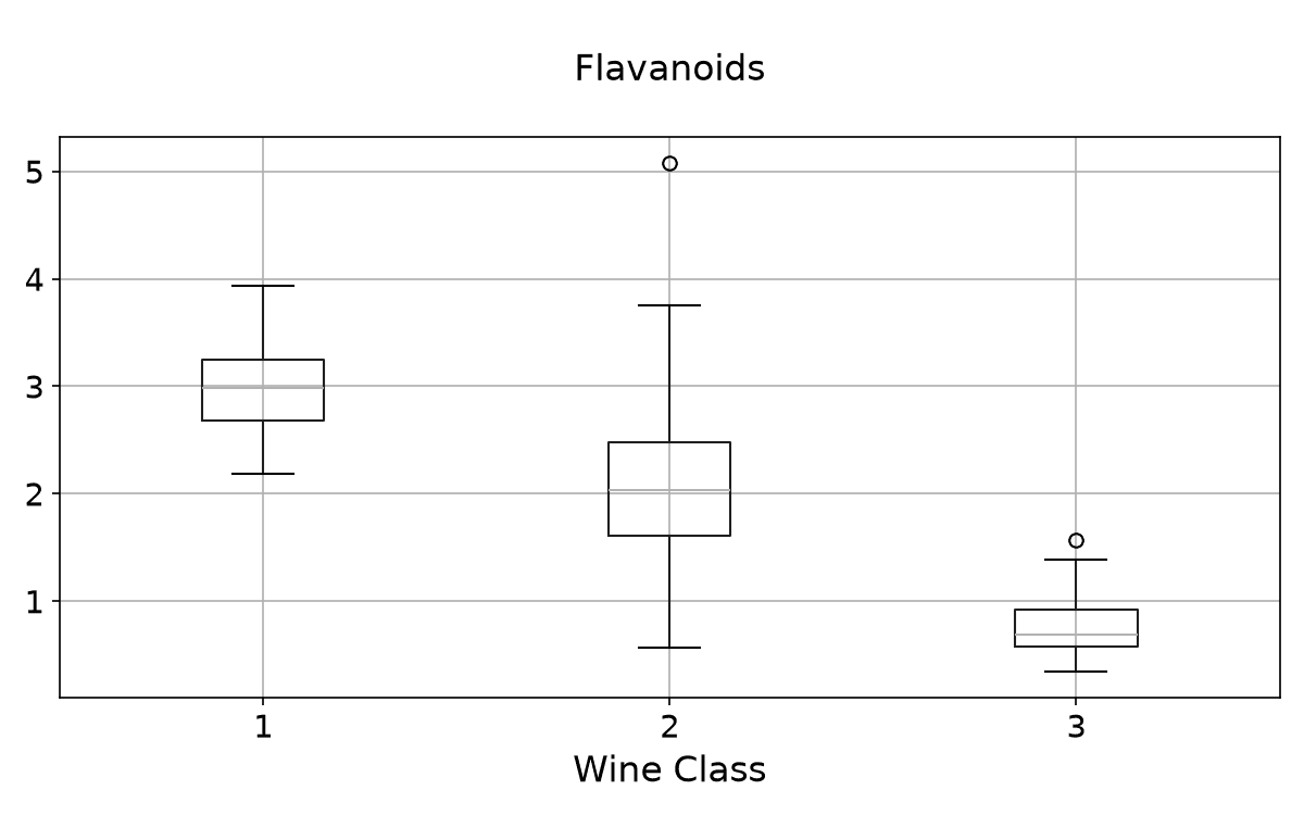
178 wines, 3 cultivars (Class 1, 2, 3: 59, 71, 48 wines), 13 numeric features such as Alcohol, Flavanoids, Proline

Boxplot of Flavanoids by wine class: class 1 highest, class 2 in the middle, class 3 lowest

python

url = ("https://raw.githubusercontent.com/tirthajyoti/"
       "Machine-Learning-with-Python/master/"
       "Datasets/wine.data.csv")
df = pd.read_csv(url)

Notebook 2 reads ./Datasets/wine.data.csv, which is not next to it in Colab. Its Colab link is on the lesson page.

Are the Features Independent?

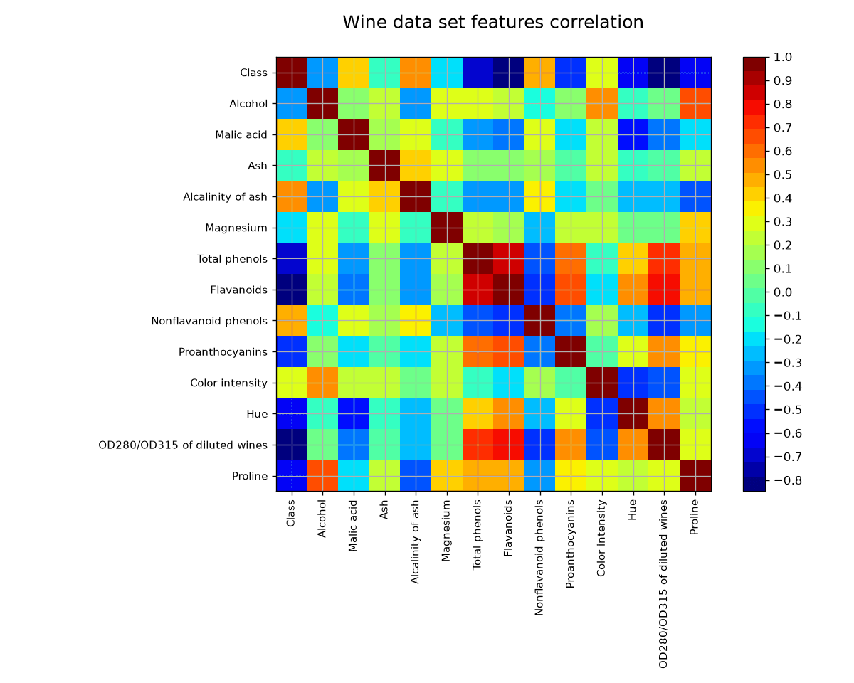
Correlation matrix of the wine columns with strong red blocks between Total phenols, Flavanoids and OD280/OD315

Flavanoids vs Total phenols: correlation 0.86
Flavanoids vs OD280/OD315: 0.79
The naive assumption is clearly false here

The Gaussian Likelihood

Inside each class, a feature is assumed to follow a bell curve

f(x | c) = 1√(2πσ_c²) · e^{-(x - μ_c)² / (2σ_c²)}

Symbol	Meaning
`μ_c`	mean of the feature in class `c`
`σ_c`	standard deviation of the feature in class `c`
`f(x \| c)`	height of the curve at `x`: the likelihood

By hand

Worked Example: One Wine, One Feature

Flavanoids over all 178 wines

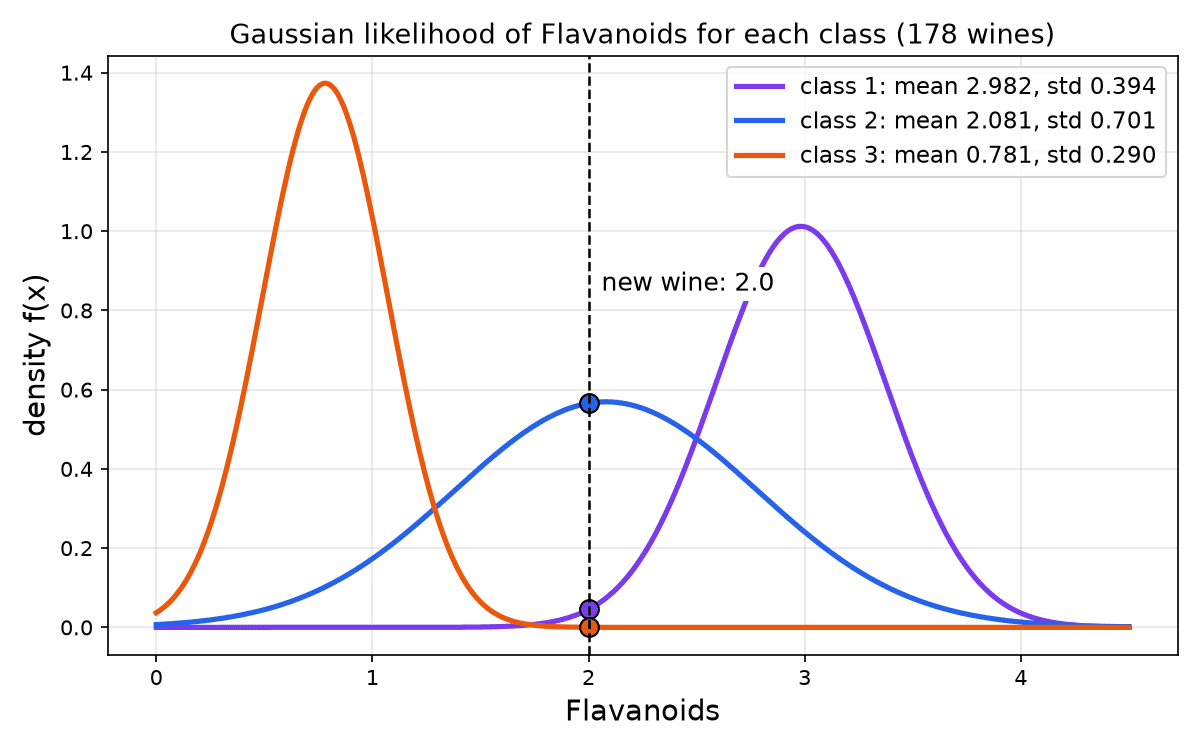
Class	Wines	Mean `μ`	Std `σ`
1	59	2.982	0.394
2	71	2.081	0.701
3	48	0.781	0.290

Step 1: The Exponents

Exponent: -(x - μ)^2 / (2σ^2) with x = 2.0

c = 1: - (2.0 - 2.982)²2 · 0.394² = - 0.96430.3105 = -3.106

c = 2: - (2.0 - 2.081)²2 · 0.701² = - 0.006560.9828 = -0.0067

c = 3: - (2.0 - 0.781)²2 · 0.290² = - 1.48600.1682 = -8.834

Step 2: The Densities

Multiply e to the exponent by 1 / √(2πσ²)

f(2.0 | 1) = 1.0125 × 0.04478 = 0.0453

f(2.0 | 2) = 0.5691 × 0.99335 = 0.5653

f(2.0 | 3) = 1.3757 × 0.000146 = 0.000200

The three Gaussian curves of Flavanoids per class, with the new wine at 2.0 marked on each curve

Step 3: Priors and the Posterior

Priors: 59/178, 71/178, 48/178

Class	f(x \| c)	P(c)	Posterior
1	0.0453	0.3315	0.0625
2	0.5653	0.3989	0.9373
3	0.000200	0.2697	0.0002

Try It: Gaussian Naive Bayes

Train on All 13 Features

python

X = df.drop('Class', axis=1)
y = df['Class']
X_train, X_test, y_train, y_test = train_test_split(
    X, y, test_size=0.3, random_state=0)

nbc = GaussianNB()
nbc.fit(X_train, y_train)
y_pred = nbc.predict(X_test)

	Pred 1	Pred 2	Pred 3
True 1	19	0	0
True 2	2	19	1
True 3	0	0	13

A Swapped Report

The notebook prints classification_report(y_pred, y_test)

Call	Precision	Recall	Support
`(y_pred, y_test)`	0.86	1.00	19
`(y_test, y_pred)`	1.00	0.86	22

Before you practise

Common Mistakes

Reading the data from a folder that does not exist in Colab
Calling plot_confusion_matrix: use ConfusionMatrixDisplay.from_estimator
alpha=0: one unseen word sets a class probability to exactly 0
fit_transform on new e-mails: new text needs vectorizer.transform([...])
Swapping classification_report arguments: true labels first
MultinomialNB on measurements: counts to Multinomial, numbers to Gaussian

Your team project

Project Milestone: Model Implementation

Pick the variant: MultinomialNB for word counts, GaussianNB for numeric features
Split with a fixed random_state
Fit, then predict the test set
Report the confusion matrix and classification_report (true labels first)
Compare with your week 5 and 6 models on the same split, and keep the best

Part 5

Practice: Your Turn

About 5 minutes

Practice 1: Bayes for Two More Words

Word	Spam e-mails (of 500)	Ham e-mails (of 499)
`click`	50	6
`meeting`	1	89

P(S | k) = 0.1 × 0.50050.056056 = 0.8929 = 5056

P(S | g) = 0.002 × 0.50050.09009 = 0.0111 = 190

About 10 minutes

Practice 2: The Four-Word Filter

e: Make money online, no meeting needed

s(H) = 0.4995 × 0.1931 × 0.0396 × 0.7624 = 0.002912

s(S) = 0.5005 × 0.5493 × 0.3345 × 0.00704 = 0.0006474

P(S | e) = 0.00064740.002912 + 0.0006474 = 0.1819

About 5 minutes

Practice 3: Gaussian by Hand

Class	f(x \| c)	P(c)	Score
1	0.4791	0.3315	0.1588
2	0.4760	0.3989	0.1899

About 10 minutes

Practice 4: In Colab

Run notebook 1 with the two fixes
Classify three e-mails with one call to predict and one to predict_proba: the code review, the meds e-mail, Make money online, no meeting needed
Why does the third one differ from Practice 2? Print inverse_transform
Notebook 2: random_state 1, then 42. How many wines are mislabelled?

Question	Result
`predict` on the batch	`[0 1 1]`, third: `P(S) = 0.7002`
Third e-mail's words	`make`, `make money`, `meeting`, `money`, `needed`, `online`
`random_state=1` / `42`	1 and 0 of 54 mislabelled

Key Takeaways

Bayes' theorem turns a countable likelihood into the posterior we want
The naive assumption: the likelihood of an e-mail is a product over its words
Predict the class with the largest prior times likelihoods; normalize for probabilities
Laplace smoothing (alpha=1) stops one unseen word from forcing a 0
MultinomialNB for word counts, GaussianNB for numeric features
It trains by counting: fast, and good even when the assumption is false

Open this lesson

Mahmoud AbasNaive Bayes Classification