Types of sequence problems

14 min read

Lesson slides

1 / 16

Types of Sequence Problems

Recurrent Neural Networks: why order matters, sequence problem types, and RNN, GRU, LSTM architectures

Recurrent Neural Networks

The main idea behind recurrent neural networks is that the input is fed to them sequentially through time.

for example the feed forward neural network would work in the following way.

feed forward network

In the network above, each word is feed to an activation function, regardless of it's order, the activation function has no clue what word have been seen before or after, as the output of the activation is calculated as

$h1(x) = h1('product', 'was', 'not', 'good') = W_{1,1} * 'product' + W_{1,2} * 'was' + W_{1,3}*'not'+ W_{1,4}*'good'$

And you can see here that if we changed the order of the tokens, nothing will change.

Now let's see how Recurrent networks does this

recurrent neural network

In the recurrent network, the input goes through the same hidden layer multiple times, updating it's weights, and thus taking into account the order of the inputs because it update itself based on the order of the input.

So the activation is calculated here in this example as follows

$h1(x) = {\color{Red} h1('good', } {\color{Green} h1('not',} {\color{Blue} h1('was', } {\color{Yellow} h1('product', '<sos>')}{\color{Blue} )}{\color{Green} )}{\color{Red} )}$

As you can see here each function takes as it's input the previous function, which takes into account the previous input and so on till the first input.

Types of sequence problems

source

The cases we might use sequence models might include for example:

One to Many a. song generator b. text generator
Many to One a. Sentiment Analysis b. Voice verification (like to tell if this is person X or not)
Many to Many (in the same time) a. Named Entities recognition b. Part of Speech tagging
Many to Many (encoder-decoder) a. Machine translation b. Question Answering

for one to one we don't need sequence model

What happens inside the RNN block ??

source

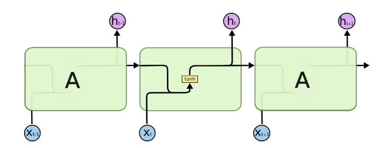
The cell by itself does one calculation, which is the hidden state $h_t$ , in some cases the output of this cell is fed to a sigmoid or a softmax output and this would be another output called $a_t$

Deal with RNN inputs

We need to pad all the inputs of the RNN so that they all have the same length or time so to speak, for example if one input is 'the product was very good with few problems' would have 8 steps, for the next input let's say its: 'a good product' this one have only 3 steps, so we pad it with 5 more tokens to make it in the same length as our longest sentence so it would be like so 'a good product <PAD> <PAD> <PAD> <PAD> <PAD>'.

Input representation

We represent our input in this case in embeddings, in the same way we discussed before, either character level or word or even sentence level.

Of course we can make use of a pre-trained model to generate these embeddings for us.

Multi layer RNN ?

The RNN cell can be stacked up to build multilayer network, let's see how it will look.

As you can see, each input passes through the first layer then the second layer, thus will enable the second layer to build a complex representation upon the first one's.

Can we see the future ?

We solved the problem of input order, but can't we make use of the future inputs, because for example we might make use of the later text in our input to classify the current text.

Bidirectional Recurrent Neural Network BiRNN

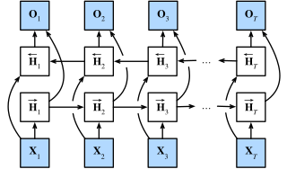
The main idea of the bidirectional rnn is to capture both the inputs from the past and the future, note here that we can't drive the output of the network till all of the inputs were loaded, in another words, you can't get a many to many model in a way that on each input word you got a label.

Building RNN with Tensorflow

Embedding layer

The embedding layer is used to generate embeddings for tokens as they are fed to the network, remember what we did in the embedding step before?

## Load the data to get started
import pandas as pd
import numpy as np
 
import tensorflow as tf

word2idx = tf.keras.datasets.imdb.get_word_index()
(x_train, y_train), (x_test, y_test) = tf.keras.datasets.imdb.load_data()

x_train[1][1]

idx2word = {word2idx[word]: word for word in word2idx.keys()}

idx2word[194]

'thought'

# tokens = [1, 14, 22, 43]
# => "<start> movie was great"
def reconstruct(tokens):
    text = []
    for token in tokens:
        text.append(idx2word[token])
    return " ".join(text)

x_train[0]

x_train.shape

(25000,)

reconstruct(x_train[0])

"the as you with out themselves powerful lets loves their becomes reaching had journalist of lot from anyone to have after out atmosphere never more room titillate it so heart shows to years of every never going villaronga help moments or of every chest visual movie except her was several of enough more with is now current film as you of mine potentially unfortunately of you than him that with out themselves her get for was camp of you movie sometimes movie that with scary but pratfalls to story wonderful that in seeing in character to of 70s musicians with heart had shadows they of here that with her serious to have does when from why what have critics they is you that isn't one will very to as itself with other tricky in of seen over landed for anyone of gilmore's br show's to whether from than out themselves history he name half some br of 'n odd was two most of mean for 1 any an boat she he should is thought frog but of script you not while history he heart to real at barrel but when from one bit then have two of script their with her nobody most that with wasn't to with armed acting watch an for with heartfelt film want an"

y_train[1]

## In case you have multi-labeles
## We need to decode y here
# y_train_encoded = tf.keras.utils.to_categorical(y_train)
# y_test_encoded = tf.keras.utils.to_categorical(y_test)

Let' pad x_train to make sure they are all of the same length

len(x_train[0]), len(x_train[1])

(218, 189)

max_sequence_len = 0
for sentence in x_train:
    max_sequence_len = max(len(sentence), max_sequence_len)
print(max_sequence_len)

Because this max length is too much, let's make it up to 100

max_sequence_len = 100

Now let's padd all the sentences to have that max length

x_train_padded = np.zeros((x_train.shape[0], max_sequence_len))
for i, sent in enumerate(x_train):
    x_train_padded[i, :len(sent)] = sent[:max_sequence_len]

x_train_padded.shape

(25000, 100)

the same for x_test

x_test_padded = np.zeros((x_test.shape[0], max_sequence_len))
for i, sent in enumerate(x_test):
    x_test_padded[i, :len(sent)] = sent[:max_sequence_len]
x_test_padded.shape

(25000, 100)

Now let's build the model

# check the vocabulary size
len(word2idx)

VOCAB_SIZE = len(word2idx)
print(VOCAB_SIZE)
embedding_dim = 100

model = tf.keras.models.Sequential([
    tf.keras.layers.Embedding(input_dim=VOCAB_SIZE+1, output_dim=embedding_dim,),
    tf.keras.layers.SimpleRNN(64),
    tf.keras.layers.Dense(64, activation='relu'),
    tf.keras.layers.Dense(1, activation='sigmoid')
])

model.compile(loss=tf.keras.losses.BinaryCrossentropy(),
              optimizer=tf.keras.optimizers.Adam(),
              metrics=['accuracy'])

model.summary()

Model: "sequential"
_________________________________________________________________
 Layer (type)                Output Shape              Param #   
=================================================================
 embedding (Embedding)       (None, None, 100)         8858500   
                                                                 
 simple_rnn (SimpleRNN)      (None, 64)                10560     
                                                                 
 dense (Dense)               (None, 64)                4160      
                                                                 
 dense_1 (Dense)             (None, 1)                 65        
                                                                 
=================================================================
Total params: 8,873,285
Trainable params: 8,873,285
Non-trainable params: 0
_________________________________________________________________

history = model.fit(x_train_padded, y_train, epochs=5,
                    validation_data=(x_test_padded, y_test),
                    validation_steps=30)

Epoch 1/5
782/782 [==============================] - 137s 173ms/step - loss: 0.6962 - accuracy: 0.5051 - val_loss: 0.6948 - val_accuracy: 0.5008
Epoch 2/5
782/782 [==============================] - 135s 173ms/step - loss: 0.6613 - accuracy: 0.5995 - val_loss: 0.6155 - val_accuracy: 0.6730
Epoch 3/5
782/782 [==============================] - 135s 172ms/step - loss: 0.5100 - accuracy: 0.7518 - val_loss: 0.6360 - val_accuracy: 0.7232
Epoch 4/5
782/782 [==============================] - 135s 172ms/step - loss: 0.4097 - accuracy: 0.8163 - val_loss: 0.6980 - val_accuracy: 0.5725
Epoch 5/5
782/782 [==============================] - 138s 176ms/step - loss: 0.4244 - accuracy: 0.7978 - val_loss: 0.7872 - val_accuracy: 0.6220

test_loss, test_acc = model.evaluate(x_test_padded, y_test)
 
print('Test Loss: {}'.format(test_loss))
print('Test Accuracy: {}'.format(test_acc))

782/782 [==============================] - 5s 6ms/step - loss: 0.7970 - accuracy: 0.5984
Test Loss: 0.7969642877578735
Test Accuracy: 0.598360002040863

Can we make it work in both directions ?

model_bi = tf.keras.models.Sequential([
    tf.keras.layers.Embedding(VOCAB_SIZE, 64),
    tf.keras.layers.Bidirectional(tf.keras.layers.SimpleRNN(64)),
    tf.keras.layers.Dense(64, activation='relu'),
    tf.keras.layers.Dense(1, activation='sigmoid')
])

model_bi.compile(loss=tf.keras.losses.BinaryCrossentropy(),
              optimizer=tf.keras.optimizers.Adam(),
              metrics=['accuracy'])

history = model_bi.fit(x_train_padded, y_train, epochs=5,
                    validation_data=(x_test_padded, y_test),
                    validation_steps=30)

test_loss, test_acc = model_bi.evaluate(x_test_padded, y_test)
 
print('Test Loss: {}'.format(test_loss))
print('Test Accuracy: {}'.format(test_acc))

Ops, i forgot !

One of the RNN drawback is that it tends to forget what it saw early in the sequence, because it will vanish eventually.
Also the gradient of the RNN cell is very likely to vanish or explode.

To solve these issue, two different versions of the SimpleRNN were proposed.

Gated Recurrent Unit (GRU)

The GRU cell replaces the Simple rnn cell, and adds a gate to the network, this gates allows the network to choose what to keep from the previous state, and thus can keep track of some memories, and also solves the vanishing gradient problem.

Without much math details, the gates here allows to forget certain points of the hidden states.

The simplified version of the equations are as follows

Here we say that $C^t = a^t = h^t$ meaning that that output state/hidden state are the same

The parameter $\tilde{C}$ is the candidate to replace vector, which will include the candidate hidden state

$\tilde{C} = tanh(W_c [C^{t-1}, X^t] + b_c)$

The gate $\Gamma_u$ is the gate that will tell which to forget of the last state and which to remember.

$\Gamma_u = \sigma(W_u [C^{t-1}, X^t] + b_u)$

The parameter $C^t$ includes the final output of the cell

$C^t = \Gamma_u*\tilde{C} + (1-\Gamma_u)* C^{t-1}$

So:

if $\Gamma_u=0$ then $C^t = C^{t-1}$
if $\Gamma_u=1$ then $C^t = \tilde{C}$

Implementing GRU in Tensorflow

The implementation will be as simple as replacing one line of the code above

gru_bi = tf.keras.models.Sequential([
    tf.keras.layers.Embedding(VOCAB_SIZE, 64),
    tf.keras.layers.Bidirectional(tf.keras.layers.GRU(64, return_sequences=True)),
    tf.keras.layers.Bidirectional(tf.keras.layers.GRU(64)),
    tf.keras.layers.Dense(64, activation='relu'),
    tf.keras.layers.Dense(1, activation='sigmoid')
])

gru_bi.compile(loss=tf.keras.losses.BinaryCrossentropy(),
              optimizer=tf.keras.optimizers.Adam(),
              metrics=['accuracy'])

history = gru_bi.fit(x_train_padded, y_train, epochs=5,
                    validation_data=(x_test_padded, y_test),
                    validation_steps=30)

test_loss, test_acc = gru_bi.evaluate(x_test_padded, y_test)
 
print('Test Loss: {}'.format(test_loss))
print('Test Accuracy: {}'.format(test_acc))

Looong sequences

There is one more important architecture that you need to know before we wrap up, the LSTM

Long Short Term Memory (LSTM)

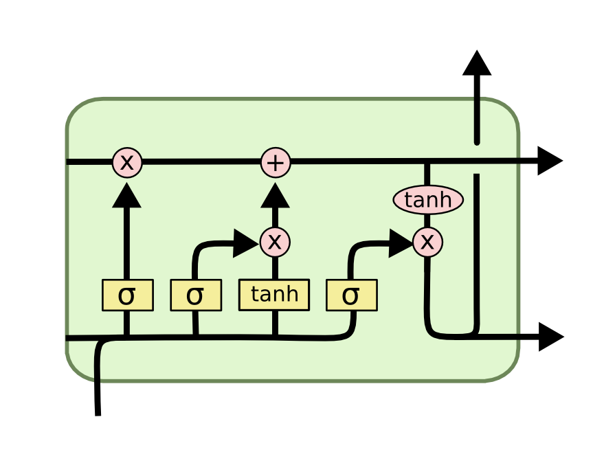
The lstm offers a long term memory component beside the short term one, and thus enables your model to remember things that he have seen way far in the past, let's go through the idea of the LSTM.

First the candidate new memory is calculated via the following equation

$\tilde{C} = tanh(W_c [a^{t-1}, x^t] + b_c)$

Here we simply take the last activation output (or the short term memory) and calculate what is the candidate of it to be remembered.

Then we have three gates here, update, forget and output, let's examine their equations.

update gate $\Gamma_u = \sigma(W_u [a^{t-1}, x^t] + b_u)$

forget gate $\Gamma_f = \sigma(W_f [a^{t-1}, x^t] + b_f)$

output gate $\Gamma_o = \sigma(W_o [a^{t-1}, x^t] + b_o)$

So the three gates learn to remember, forget and update which parts of the hidden state, thus enable our model to work with relatively long sequences.

Now to the outputs of our cell

the long term memory $C^t = \Gamma_u*\tilde{C} + \Gamma_f*C^{t-1}$

So basically update these new values that i have just learned $\Gamma_u*\tilde{C}$ ,and keep from the last memory what the forget gate tells you $\Gamma_f*C^{t-1}$

the short term memory $a^t = \Gamma_o*tanh(C^t)$

just an activation function applied to the short memory learned in this step, and of course based only on the output of the $\Gamma_o$ gate.

the output for this cell (aka prediction) $y^t = softmax(w_y.a^t + b_y)$

And these together allows the LSTM to work with the large sequences without forgetting what was in the very first of the sentence, thus it can work with long sequences.

Bidirectional LSTMs

The idea is the same as in RNN and GRU, the only difference is that we change the rnn block to LSTM block!

Long sequence ?

Now we can let go the sequence length that we limited above !

max_sequence_len = 0
for sentence in x_train:
    max_sequence_len = max(len(sentence), max_sequence_len)
print(max_sequence_len)

x_train_padded = np.zeros((x_train.shape[0], max_sequence_len))
for i, sent in enumerate(x_train):
    x_train_padded[i, :len(sent)] = sent[:max_sequence_len]

x_train_padded.shape

the same for x_test

x_test_padded = np.zeros((x_test.shape[0], max_sequence_len))
for i, sent in enumerate(x_test):
    x_test_padded[i, :len(sent)] = sent[:max_sequence_len]
x_test_padded.shape

lstm_bi = tf.keras.models.Sequential([
    tf.keras.layers.Embedding(VOCAB_SIZE, 64),
    tf.keras.layers.Bidirectional(tf.keras.layers.LSTM(64)),
    tf.keras.layers.Dense(64, activation='relu'),
    tf.keras.layers.Dense(1, activation='sigmoid')
])

lstm_bi.compile(loss=tf.keras.losses.BinaryCrossentropy(),
              optimizer=tf.keras.optimizers.Adam(),
              metrics=['accuracy'])

history = lstm_bi.fit(x_train_padded, y_train, epochs=5,
                    validation_data=(x_test_padded, y_test),
                    validation_steps=30)

test_loss, test_acc = lstm_bi.evaluate(x_test_padded, y_test)
 
print('Test Loss: {}'.format(test_loss))
print('Test Accuracy: {}'.format(test_acc))

run the next cell to store the models

How can we predict an input given these models ?

# save the lstm model
lstm_bi.save('models/lstm_bi')

## Load the data
import tensorflow as tf
import numpy as np
 
lstm_padding = 2494
 
word2idx = tf.keras.datasets.imdb.get_word_index()
 
lstm_bi = tf.keras.models.load_model('models/lstm_bi')

def predict(text, clf, word2idx, padding_size):
    # padd the text
    padded_text = np.zeros((padding_size))
 
    # transform your text into indices
    padded_text[:min(padding_size, len(text.split()))] = [
        word2idx.get(word, 0) for word in text.split()][:padding_size]
 
    # predict it !
    prediction = clf.predict(tf.expand_dims(padded_text, 0)) # expand_dims to add the batch dimension
    # padded_text → [23, 55, 812, 4, 0, 0, 0]     # shape: (7,)
    # tf.expand_dims(padded_text, 0) → [[23, 55, 812, 4, 0, 0, 0]]    # shape: (1, 7)
 
    return prediction

text= "the movie was super awesome!"

predict(text, lstm_bi, word2idx, lstm_padding)

text2= "the movie was bad and ugly"

predict(text2, lstm_bi, word2idx, lstm_padding)

Conclusion

In this notebook we have seen a brief on the recurrent neural networks, how they work and how to deal with sequences using them.

We have seen that RNN are much more efficient in working with sequences because they learn the knowledge embedded in the sequence unlike feed forward network.

We also discussed how GRU is better than RNN in two main points, the way it handles the memory and also the vanishing gradient handling.

Finally we have seen the LSTM and how it adds more gates to learn more about the sequence and enable a long term memory besides the short term, thus can work with larger sequences.

Types of Sequence Problems

Recurrent Neural Networks

Types of sequence problems

What happens inside the RNN block ??

Deal with RNN inputs

Input representation

Multi layer RNN ?

Can we see the future ?

Bidirectional Recurrent Neural Network BiRNN

Building RNN with Tensorflow

Embedding layer

Let' pad x_train to make sure they are all of the same length

Now let's build the model

Can we make it work in both directions ?

Ops, i forgot !

Gated Recurrent Unit (GRU)

Implementing GRU in Tensorflow

Looong sequences

Long Short Term Memory (LSTM)

Bidirectional LSTMs

Long sequence ?

How can we predict an input given these models ?

Conclusion

Good readings