أنواع مسائل المتتاليات (Sequence Problems)

13 دقيقة قراءة

شرائح الدرس

1 / 16

أنواع مسائل المتتاليات

الشبكات العصبية المتكررة (RNN): لماذا يهم الترتيب، وأنواع مسائل المتتاليات، ومعماريات RNN وGRU وLSTM

الشبكات العصبية التكرارية (Recurrent Neural Networks)

الفكرة الأساسية وراء الشبكات العصبية التكرارية (RNN) هي أن المُدخل يُغذَّى إليها بالتتابع عبر الزمن.

فمثلًا، تعمل الشبكة العصبية الأمامية (Feed Forward Neural Network) على النحو التالي.

شبكة أمامية التغذية (Feed Forward Network)

في الشبكة أعلاه، تُغذَّى كل كلمة إلى دالة تنشيط (Activation Function) بغض النظر عن ترتيبها؛ فدالة التنشيط لا تعرف أي كلمة سبقتها أو تلتها، إذ يُحسب ناتج التنشيط كالتالي:

$h1(x) = h1('product', 'was', 'not', 'good') = W_{1,1} * 'product' + W_{1,2} * 'was' + W_{1,3}*'not'+ W_{1,4}*'good'$

ويمكنك أن ترى هنا أنه لو غيّرنا ترتيب الرموز (Tokens)، فلن يتغيّر شيء.

الآن، لنرَ كيف تتعامل الشبكات التكرارية مع هذه المسألة.

شبكة عصبية تكرارية (Recurrent Neural Network)

في الشبكة التكرارية، يمرّ المُدخل عبر الطبقة المخفية (Hidden Layer) نفسها عدة مرات، محدِّثًا أوزانها في كل مرة، ومن ثمّ يأخذ في الحسبان ترتيب المدخلات لأنه يحدّث نفسه اعتمادًا على هذا الترتيب.

لذا يُحسب التنشيط هنا، في هذا المثال، على النحو التالي:

$h1(x) = {\color{Red} h1('good', } {\color{Green} h1('not',} {\color{Blue} h1('was', } {\color{Yellow} h1('product', '<sos>')}{\color{Blue} )}{\color{Green} )}{\color{Red} )}$

كما ترى هنا، تأخذ كل دالة كمُدخل الدالة السابقة لها، والتي تأخذ بدورها في الحسبان المُدخل الذي قبلها، وهكذا حتى المُدخل الأول.

أنواع مسائل المتتاليات (Sequence Problems)

المصدر

من الحالات التي قد نستخدم فيها نماذج المتتاليات (Sequence Models) على سبيل المثال:

واحد إلى عدة (One to Many) أ. مولّد الأغاني ب. مولّد النصوص
عدة إلى واحد (Many to One) أ. تحليل المشاعر (Sentiment Analysis) ب. التحقق الصوتي (Voice Verification) (مثل تحديد ما إذا كان هذا الصوت للشخص X أم لا)
عدة إلى عدة (في الوقت نفسه) أ. التعرّف على الكيانات المسمّاة (Named Entity Recognition) ب. وسم أجزاء الكلام (Part of Speech Tagging)
عدة إلى عدة (بنية المُرمِّز - المُفكِّك Encoder-Decoder) أ. الترجمة الآلية (Machine Translation) ب. الإجابة عن الأسئلة (Question Answering)

أما حالة واحد إلى واحد فلا نحتاج فيها إلى نموذج متتاليات.

ماذا يحدث داخل وحدة RNN؟

المصدر

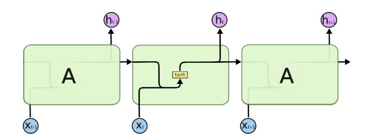
تقوم الخلية بحساب واحد بمفردها، وهو الحالة المخفية (Hidden State) $h_t$ ، وفي بعض الحالات يُغذَّى ناتج هذه الخلية إلى دالة سيغمويد (Sigmoid) أو سوفتماكس (Softmax) فيصبح ناتجًا آخر يُسمّى $a_t$ .

التعامل مع مدخلات RNN

نحتاج إلى حشو (Padding) جميع مدخلات RNN بحيث يكون طولها (أو مدتها الزمنية) واحدًا؛ فمثلًا لو كان أحد المدخلات هو الجملة 'the product was very good with few problems' فسيكون له 8 خطوات، بينما المُدخل التالي، ولنقل إنه 'a good product'، له 3 خطوات فقط، فنحشوه بخمسة رموز إضافية ليصبح بطول أطول جملة لدينا، فيصبح على الشكل التالي: 'a good product <PAD> <PAD> <PAD> <PAD> <PAD>'.

تمثيل المُدخل

نمثّل مُدخلنا في هذه الحالة عبر التضمينات (Embeddings)، بالطريقة نفسها التي ناقشناها سابقًا، سواء على مستوى الحرف أو الكلمة أو حتى الجملة.

وبالطبع يمكننا الاستفادة من نموذج مُدرَّب سلفًا (Pre-trained Model) لتوليد هذه التضمينات بدلًا منّا.

شبكة RNN متعددة الطبقات؟

يمكن تكديس خلايا RNN فوق بعضها لبناء شبكة متعددة الطبقات، فلنرَ كيف يبدو ذلك.

كما ترى، يمرّ كل مُدخل عبر الطبقة الأولى ثم الطبقة الثانية، فتتمكّن الطبقة الثانية من بناء تمثيل أكثر تعقيدًا فوق ما بنته الطبقة الأولى.

هل يمكننا رؤية المستقبل؟

لقد حللنا مشكلة ترتيب المدخلات، لكن ألا يمكننا الاستفادة من المدخلات المستقبلية؟ فمثلًا قد نستفيد من النص اللاحق في مُدخلنا لتصنيف النص الحالي.

الشبكة العصبية التكرارية ثنائية الاتجاه (BiRNN)

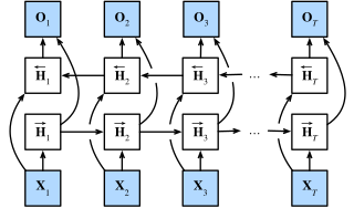
الفكرة الأساسية للشبكة التكرارية ثنائية الاتجاه هي التقاط المدخلات من الماضي والمستقبل معًا، ولاحظ هنا أننا لا نستطيع اشتقاق ناتج الشبكة إلا بعد تحميل جميع المدخلات، وبعبارة أخرى، لا يمكنك الحصول على نموذج عدة-إلى-عدة بحيث تحصل على وسم (Label) عند كل كلمة مُدخلة.

بناء شبكة RNN باستخدام Tensorflow

طبقة التضمين (Embedding Layer)

تُستخدم طبقة التضمين لتوليد تضمينات للرموز أثناء تغذيتها إلى الشبكة، أتذكر ما فعلناه في خطوة التضمين سابقًا؟

## Load the data to get started
import pandas as pd
import numpy as np
 
import tensorflow as tf

word2idx = tf.keras.datasets.imdb.get_word_index()
(x_train, y_train), (x_test, y_test) = tf.keras.datasets.imdb.load_data()

x_train[1][1]

idx2word = {word2idx[word]: word for word in word2idx.keys()}

idx2word[194]

'thought'

# tokens = [1, 14, 22, 43]
# => "<start> movie was great"
def reconstruct(tokens):
    text = []
    for token in tokens:
        text.append(idx2word[token])
    return " ".join(text)

x_train[0]

x_train.shape

(25000,)

reconstruct(x_train[0])

"the as you with out themselves powerful lets loves their becomes reaching had journalist of lot from anyone to have after out atmosphere never more room titillate it so heart shows to years of every never going villaronga help moments or of every chest visual movie except her was several of enough more with is now current film as you of mine potentially unfortunately of you than him that with out themselves her get for was camp of you movie sometimes movie that with scary but pratfalls to story wonderful that in seeing in character to of 70s musicians with heart had shadows they of here that with her serious to have does when from why what have critics they is you that isn't one will very to as itself with other tricky in of seen over landed for anyone of gilmore's br show's to whether from than out themselves history he name half some br of 'n odd was two most of mean for 1 any an boat she he should is thought frog but of script you not while history he heart to real at barrel but when from one bit then have two of script their with her nobody most that with wasn't to with armed acting watch an for with heartfelt film want an"

y_train[1]

## In case you have multi-labeles
## We need to decode y here
# y_train_encoded = tf.keras.utils.to_categorical(y_train)
# y_test_encoded = tf.keras.utils.to_categorical(y_test)

لنحشُ (Pad) بيانات x_train حتى تكون جميعها بالطول نفسه

len(x_train[0]), len(x_train[1])

(218, 189)

max_sequence_len = 0
for sentence in x_train:
    max_sequence_len = max(len(sentence), max_sequence_len)
print(max_sequence_len)

بما أن هذا الطول الأقصى كبير جدًا، فلنجعله 100 كحد أقصى.

max_sequence_len = 100

الآن لنحشُ جميع الجمل لتكون بهذا الطول الأقصى.

x_train_padded = np.zeros((x_train.shape[0], max_sequence_len))
for i, sent in enumerate(x_train):
    x_train_padded[i, :len(sent)] = sent[:max_sequence_len]

x_train_padded.shape

(25000, 100)

الأمر نفسه بالنسبة إلى x_test.

x_test_padded = np.zeros((x_test.shape[0], max_sequence_len))
for i, sent in enumerate(x_test):
    x_test_padded[i, :len(sent)] = sent[:max_sequence_len]
x_test_padded.shape

(25000, 100)

الآن لنبنِ النموذج

# check the vocabulary size
len(word2idx)

VOCAB_SIZE = len(word2idx)
print(VOCAB_SIZE)
embedding_dim = 100

model = tf.keras.models.Sequential([
    tf.keras.layers.Embedding(input_dim=VOCAB_SIZE+1, output_dim=embedding_dim,),
    tf.keras.layers.SimpleRNN(64),
    tf.keras.layers.Dense(64, activation='relu'),
    tf.keras.layers.Dense(1, activation='sigmoid')
])

model.compile(loss=tf.keras.losses.BinaryCrossentropy(),
              optimizer=tf.keras.optimizers.Adam(),
              metrics=['accuracy'])

model.summary()

Model: "sequential"
_________________________________________________________________
 Layer (type)                Output Shape              Param #   
=================================================================
 embedding (Embedding)       (None, None, 100)         8858500   
                                                                 
 simple_rnn (SimpleRNN)      (None, 64)                10560     
                                                                 
 dense (Dense)               (None, 64)                4160      
                                                                 
 dense_1 (Dense)             (None, 1)                 65        
                                                                 
=================================================================
Total params: 8,873,285
Trainable params: 8,873,285
Non-trainable params: 0
_________________________________________________________________

history = model.fit(x_train_padded, y_train, epochs=5,
                    validation_data=(x_test_padded, y_test),
                    validation_steps=30)

Epoch 1/5
782/782 [==============================] - 137s 173ms/step - loss: 0.6962 - accuracy: 0.5051 - val_loss: 0.6948 - val_accuracy: 0.5008
Epoch 2/5
782/782 [==============================] - 135s 173ms/step - loss: 0.6613 - accuracy: 0.5995 - val_loss: 0.6155 - val_accuracy: 0.6730
Epoch 3/5
782/782 [==============================] - 135s 172ms/step - loss: 0.5100 - accuracy: 0.7518 - val_loss: 0.6360 - val_accuracy: 0.7232
Epoch 4/5
782/782 [==============================] - 135s 172ms/step - loss: 0.4097 - accuracy: 0.8163 - val_loss: 0.6980 - val_accuracy: 0.5725
Epoch 5/5
782/782 [==============================] - 138s 176ms/step - loss: 0.4244 - accuracy: 0.7978 - val_loss: 0.7872 - val_accuracy: 0.6220

test_loss, test_acc = model.evaluate(x_test_padded, y_test)
 
print('Test Loss: {}'.format(test_loss))
print('Test Accuracy: {}'.format(test_acc))

782/782 [==============================] - 5s 6ms/step - loss: 0.7970 - accuracy: 0.5984
Test Loss: 0.7969642877578735
Test Accuracy: 0.598360002040863

هل يمكننا جعلها تعمل في الاتجاهين معًا؟

model_bi = tf.keras.models.Sequential([
    tf.keras.layers.Embedding(VOCAB_SIZE, 64),
    tf.keras.layers.Bidirectional(tf.keras.layers.SimpleRNN(64)),
    tf.keras.layers.Dense(64, activation='relu'),
    tf.keras.layers.Dense(1, activation='sigmoid')
])

model_bi.compile(loss=tf.keras.losses.BinaryCrossentropy(),
              optimizer=tf.keras.optimizers.Adam(),
              metrics=['accuracy'])

history = model_bi.fit(x_train_padded, y_train, epochs=5,
                    validation_data=(x_test_padded, y_test),
                    validation_steps=30)

test_loss, test_acc = model_bi.evaluate(x_test_padded, y_test)
 
print('Test Loss: {}'.format(test_loss))
print('Test Accuracy: {}'.format(test_acc))

يا للنسيان!

من عيوب RNN أنها تميل إلى نسيان ما رأته في وقت مبكر من المتتالية، لأن أثره يتلاشى في النهاية.
كذلك فإن تدرّج (Gradient) خلية RNN عرضة جدًا للتلاشي أو الانفجار.

ولحل هاتين المشكلتين، اقتُرحت نسختان مختلفتان من SimpleRNN.

الوحدة التكرارية البوابية (Gated Recurrent Unit - GRU)

تحلّ خلية GRU محلّ خلية RNN البسيطة، وتضيف بوابة (Gate) إلى الشبكة، وتتيح هذه البوابة للشبكة أن تختار ما تحتفظ به من الحالة السابقة، فتتمكن بذلك من تتبّع بعض الذكريات، كما تحلّ مشكلة تلاشي التدرّج.

من دون الخوض في تفاصيل رياضية كثيرة، تتيح هذه البوابات نسيان نقاط معيّنة من الحالات المخفية.

فيما يلي النسخة المبسّطة من المعادلات:

هنا نقول إن $C^t = a^t = h^t$ ، أي أن حالة الناتج/الحالة المخفية هي نفسها.

المُعامل $\tilde{C}$ هو مرشّح الاستبدال (Candidate)، الذي سيتضمن الحالة المخفية المرشّحة.

$\tilde{C} = tanh(W_c [C^{t-1}, X^t] + b_c)$

البوابة $\Gamma_u$ هي البوابة التي ستحدّد ما سيُنسى من الحالة الأخيرة وما سيُتذكَّر.

$\Gamma_u = \sigma(W_u [C^{t-1}, X^t] + b_u)$

المُعامل $C^t$ يتضمن الناتج النهائي للخلية.

$C^t = \Gamma_u*\tilde{C} + (1-\Gamma_u)* C^{t-1}$

إذن:

إذا كانت $\Gamma_u=0$ فإن $C^t = C^{t-1}$
إذا كانت $\Gamma_u=1$ فإن $C^t = \tilde{C}$

تطبيق GRU باستخدام Tensorflow

سيكون التطبيق بسيطًا بقدر استبدال سطر واحد من الكود أعلاه.

gru_bi = tf.keras.models.Sequential([
    tf.keras.layers.Embedding(VOCAB_SIZE, 64),
    tf.keras.layers.Bidirectional(tf.keras.layers.GRU(64, return_sequences=True)),
    tf.keras.layers.Bidirectional(tf.keras.layers.GRU(64)),
    tf.keras.layers.Dense(64, activation='relu'),
    tf.keras.layers.Dense(1, activation='sigmoid')
])

gru_bi.compile(loss=tf.keras.losses.BinaryCrossentropy(),
              optimizer=tf.keras.optimizers.Adam(),
              metrics=['accuracy'])

history = gru_bi.fit(x_train_padded, y_train, epochs=5,
                    validation_data=(x_test_padded, y_test),
                    validation_steps=30)

test_loss, test_acc = gru_bi.evaluate(x_test_padded, y_test)
 
print('Test Loss: {}'.format(test_loss))
print('Test Accuracy: {}'.format(test_acc))

متتاليات طويلة جدًا

بقي معمار مهم آخر ينبغي أن تعرفه قبل أن ننهي هذا الدرس، وهو LSTM.

الذاكرة الطويلة القصيرة المدى (Long Short Term Memory - LSTM)

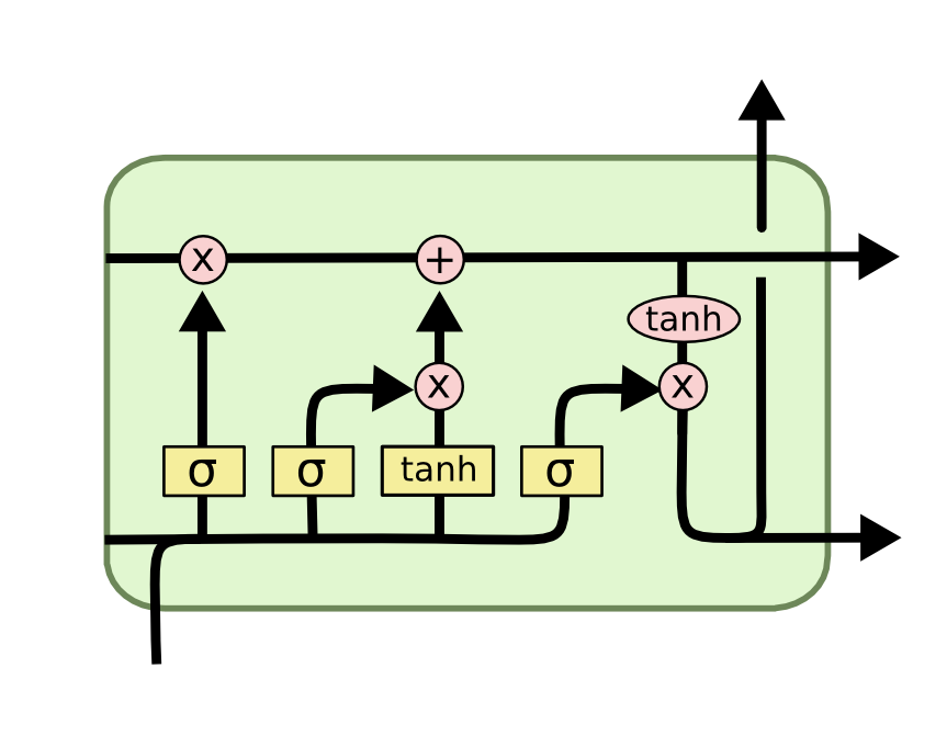
توفّر LSTM مكوّن ذاكرة طويل المدى إلى جانب المكوّن قصير المدى، فتتيح بذلك لنموذجك تذكّر أشياء رآها بعيدًا جدًا في الماضي؛ لنستعرض فكرة LSTM.

أولًا، تُحسب الذاكرة الجديدة المرشّحة عبر المعادلة التالية:

$\tilde{C} = tanh(W_c [a^{t-1}, x^t] + b_c)$

هنا نأخذ ببساطة ناتج آخر تنشيط (أو الذاكرة قصيرة المدى) ونحسب مرشّحها ليصبح ما سيُتذكَّر.

بعد ذلك لدينا ثلاث بوابات هنا: بوابة التحديث، وبوابة النسيان، وبوابة الناتج، فلنستعرض معادلاتها.

بوابة التحديث $\Gamma_u = \sigma(W_u [a^{t-1}, x^t] + b_u)$

بوابة النسيان $\Gamma_f = \sigma(W_f [a^{t-1}, x^t] + b_f)$

بوابة الناتج $\Gamma_o = \sigma(W_o [a^{t-1}, x^t] + b_o)$

فتتعلّم البوابات الثلاث إذن أن تتذكّر وتنسى وتحدّث أجزاءً من الحالة المخفية، فتتيح بذلك لنموذجنا العمل مع متتاليات طويلة نسبيًا.

الآن لنصل إلى نواتج خليتنا:

الذاكرة الطويلة المدى $C^t = \Gamma_u*\tilde{C} + \Gamma_f*C^{t-1}$

فبشكل أساسي نحدّث القيم الجديدة التي تعلّمناها للتو $\Gamma_u*\tilde{C}$ ، ونحتفظ من الذاكرة الأخيرة بما تخبرنا به بوابة النسيان $\Gamma_f*C^{t-1}$ .

الذاكرة القصيرة المدى $a^t = \Gamma_o*tanh(C^t)$

هي ببساطة دالة تنشيط تُطبَّق على الذاكرة القصيرة المتعلَّمة في هذه الخطوة، وتعتمد بالطبع فقط على ناتج بوابة $\Gamma_o$ .

ناتج هذه الخلية (أي التنبؤ) $y^t = softmax(w_y.a^t + b_y)$

وتتيح هذه العناصر مجتمعةً لِـ LSTM العمل مع المتتاليات الكبيرة من دون نسيان ما كان في بداية الجملة تمامًا، فتتمكن بذلك من التعامل مع المتتاليات الطويلة.

شبكات LSTM ثنائية الاتجاه

الفكرة نفسها الموجودة في RNN وGRU، والفرق الوحيد هو أننا نستبدل وحدة RNN بوحدة LSTM!

متتالية طويلة؟

الآن يمكننا التخلي عن حدّ طول المتتالية الذي فرضناه أعلاه!

max_sequence_len = 0
for sentence in x_train:
    max_sequence_len = max(len(sentence), max_sequence_len)
print(max_sequence_len)

x_train_padded = np.zeros((x_train.shape[0], max_sequence_len))
for i, sent in enumerate(x_train):
    x_train_padded[i, :len(sent)] = sent[:max_sequence_len]

x_train_padded.shape

الأمر نفسه بالنسبة إلى x_test.

x_test_padded = np.zeros((x_test.shape[0], max_sequence_len))
for i, sent in enumerate(x_test):
    x_test_padded[i, :len(sent)] = sent[:max_sequence_len]
x_test_padded.shape

lstm_bi = tf.keras.models.Sequential([
    tf.keras.layers.Embedding(VOCAB_SIZE, 64),
    tf.keras.layers.Bidirectional(tf.keras.layers.LSTM(64)),
    tf.keras.layers.Dense(64, activation='relu'),
    tf.keras.layers.Dense(1, activation='sigmoid')
])

lstm_bi.compile(loss=tf.keras.losses.BinaryCrossentropy(),
              optimizer=tf.keras.optimizers.Adam(),
              metrics=['accuracy'])

history = lstm_bi.fit(x_train_padded, y_train, epochs=5,
                    validation_data=(x_test_padded, y_test),
                    validation_steps=30)

test_loss, test_acc = lstm_bi.evaluate(x_test_padded, y_test)
 
print('Test Loss: {}'.format(test_loss))
print('Test Accuracy: {}'.format(test_acc))

نفّذ الخلية التالية لحفظ النماذج

كيف يمكننا التنبؤ بمُدخل باستخدام هذه النماذج؟

# save the lstm model
lstm_bi.save('models/lstm_bi')

## Load the data
import tensorflow as tf
import numpy as np
 
lstm_padding = 2494
 
word2idx = tf.keras.datasets.imdb.get_word_index()
 
lstm_bi = tf.keras.models.load_model('models/lstm_bi')

def predict(text, clf, word2idx, padding_size):
    # padd the text
    padded_text = np.zeros((padding_size))
 
    # transform your text into indices
    padded_text[:min(padding_size, len(text.split()))] = [
        word2idx.get(word, 0) for word in text.split()][:padding_size]
 
    # predict it !
    prediction = clf.predict(tf.expand_dims(padded_text, 0)) # expand_dims to add the batch dimension
    # padded_text → [23, 55, 812, 4, 0, 0, 0]     # shape: (7,)
    # tf.expand_dims(padded_text, 0) → [[23, 55, 812, 4, 0, 0, 0]]    # shape: (1, 7)
 
    return prediction

text= "the movie was super awesome!"

predict(text, lstm_bi, word2idx, lstm_padding)

text2= "the movie was bad and ugly"

predict(text2, lstm_bi, word2idx, lstm_padding)

الخاتمة

استعرضنا في هذا الدرس نبذة عن الشبكات العصبية التكرارية، وكيف تعمل، وكيفية التعامل مع المتتاليات باستخدامها.

رأينا أن شبكات RNN أكثر كفاءة بكثير في العمل مع المتتاليات لأنها تتعلّم المعرفة المُضمَّنة في المتتالية، بخلاف الشبكة الأمامية التغذية.

كما ناقشنا كيف تتفوّق GRU على RNN من ناحيتين أساسيتين: طريقة تعاملها مع الذاكرة، وكذلك معالجتها لمشكلة تلاشي التدرّج.

وأخيرًا استعرضنا LSTM وكيف تضيف مزيدًا من البوابات لتتعلّم أكثر عن المتتالية وتتيح ذاكرة طويلة المدى إلى جانب القصيرة المدى، فتتمكن بذلك من العمل مع متتاليات أكبر.

أنواع مسائل المتتاليات

الشبكات العصبية التكرارية (Recurrent Neural Networks)

أنواع مسائل المتتاليات (Sequence Problems)

ماذا يحدث داخل وحدة RNN؟

التعامل مع مدخلات RNN

تمثيل المُدخل

شبكة RNN متعددة الطبقات؟

هل يمكننا رؤية المستقبل؟

الشبكة العصبية التكرارية ثنائية الاتجاه (BiRNN)

بناء شبكة RNN باستخدام Tensorflow

طبقة التضمين (Embedding Layer)

لنحشُ (Pad) بيانات x_train حتى تكون جميعها بالطول نفسه

الآن لنبنِ النموذج

هل يمكننا جعلها تعمل في الاتجاهين معًا؟

يا للنسيان!

الوحدة التكرارية البوابية (Gated Recurrent Unit - GRU)

تطبيق GRU باستخدام Tensorflow

متتاليات طويلة جدًا

الذاكرة الطويلة القصيرة المدى (Long Short Term Memory - LSTM)

شبكات LSTM ثنائية الاتجاه

متتالية طويلة؟

كيف يمكننا التنبؤ بمُدخل باستخدام هذه النماذج؟

الخاتمة

قراءات مفيدة